

InferenceX v2: NVIDIA Blackwell Vs AMD vs Hopper - Formerly InferenceMAX
GB300 NVL72, MI355X, B200, H100, Disaggregated Serving, Wide Expert Parallelism, Large Mixture of Experts, SGLang, vLLM, TRTLLM
Introduction
InferenceXv2 (formerly InferenceMAX) builds on the foundation established by InferenceMAXv1, our open-source, continuously updated inference benchmark that has set a new standard for AI inference performance and economics. InferenceMAXv1 moved beyond static, point-in-time benchmarks by running continuous tests across hundreds of chips and popular open-source frameworks. Free dashboard available here.
Our benchmark has been widely reproduced, validated and/or supported by almost every major buyer of compute from Google Cloud to Microsoft Azure to Oracle, OpenAI, and many more.
InferenceXv2 builds on this foundation. It expands coverage to include large scale DeepSeek MoE disaggregated inference (disagg prefill, or simply “disagg”) with wide expert parallelism (wideEP) optimization to all 6 NVIDIA western GPU SKUs from the past 4 years as well as to every single AMD western GPU SKU released in the past 3 years – in total InferenceXv2 utilizes close to 1000 frontier GPUs for a full benchmark run across all SKUs.
With today’s release, InferenceXv2 is now the first suite to benchmark the Blackwell Ultra GB300 NVL72 and B300 across the whole pareto frontier curve, and it is the first third party benchmark to test disagg+wideEP multi-node FP4 and FP8 MI355X performance. In future iterations of InferenceX, we will continue to focus heavily on disaggregated serving with wide expert parallelism as that is what is deployed in production at Frontier AI Labs like OpenAI, Anthropic, xAI, Google Deepmind, DeepSeek as well as advanced API providers like TogetherAI, Baseten, and Fireworks. In this article, we will also break down the system engineering principles and economics in play around the latest Claude Code Fast mode feature.
Our benchmark is completely open-source under Apache 2.0 – this means that we are able to move at the same rapid speed at which the AI software ecosystem is advancing. If you like our work and would like to show us some support, please drop a star on our GitHub! We also provide a free data visualizer at https://inferencex.com for everyone in the ML community to explore the complete dataset themselves.
We will add DeepSeekv4 and other popular Chinese frontier models with day 0 support as over the past 6 months, we now have cleaned up a lot of tech debt and are able to move fast with stable infrastructure. We will also be adding TPUv7 Ironwood and Trainium3 to InferenceX later this year! If you want to contribute to our impactful mission while earning a competitive compensation, consider applying here.
Key Observations and Results to Highlight
We see competitive perf per TCO results on FP8 MI355X disagg+wideEP SGLang on AMD compared to FP8 B200 disagg+wideEP SGLang, but when compared to widely used Dynamo TRTLLM B200 FP8, TRT continues to framemog. This is amazing news that AMD SGLang Disagg prefill+wideEP for FP8 is able to match NVIDIA’s SGLang performance.
We also see that for single node aggregated serving, AMD’s SGLang delivers better perf per TCO than NVIDIA’s SGLang for FP8. It is also great to see that AMD has deprecated their second class fork of vllm to move further upstream and closer to delivering first class experience. Stay tuned for our “State of AMD” article where we talk about the many areas where AMD’s pace of improvement has been rapid & also the areas where the pace of improvement has been lackluster. We recommend that NVIDIA focus even more on SGLang & vLLM ecosystem in addition their TRTLLM engine. Jensen needs to staff more resources & engineers towards contributing open ecosystems like SGLang & vLLM.
When it comes to the latest inference techniques that are used by the most prominent frontier large-scale inference services (such as disagg prefill+wideEP+FP4), Nvidia absolutely frame mogs with the B200, B300 and ASU frat leader, rack scale GB200/GB300 NVL72 across both SGLang and TRTLLM. Nvidia GPUs also dominate when it comes to energy efficiency, with much lower all-in provisioned picoJoules of energy per token across all workloads.
Turning to AMD, we find that the biggest issue with inference on their systems and using their software is composability. That is, many of AMDs inference optimization implementations work well in isolation, but when combined with other optimizations, the result is not as competitive as one would expect. Specifically, the composability of disagg prefill, wideEP and FP4 inference optimizations needs significant improvement.
While performance is competitive on AMD when enabling just a subset of the SOTA inference optimizations, enabling all three major optimizations that labs use, AMD’s performance is currently not competitive with Nvidia’s. We strongly recommend to AMD that they focus heavily on composability of different inference optimizations. We have been told that AMD will start focusing on software composability of FP4+distributed inferencing across their whole software stack. This will happen after Chinese New Year as most of their disagg prefill+wideEP 10x inference engineers are based in China
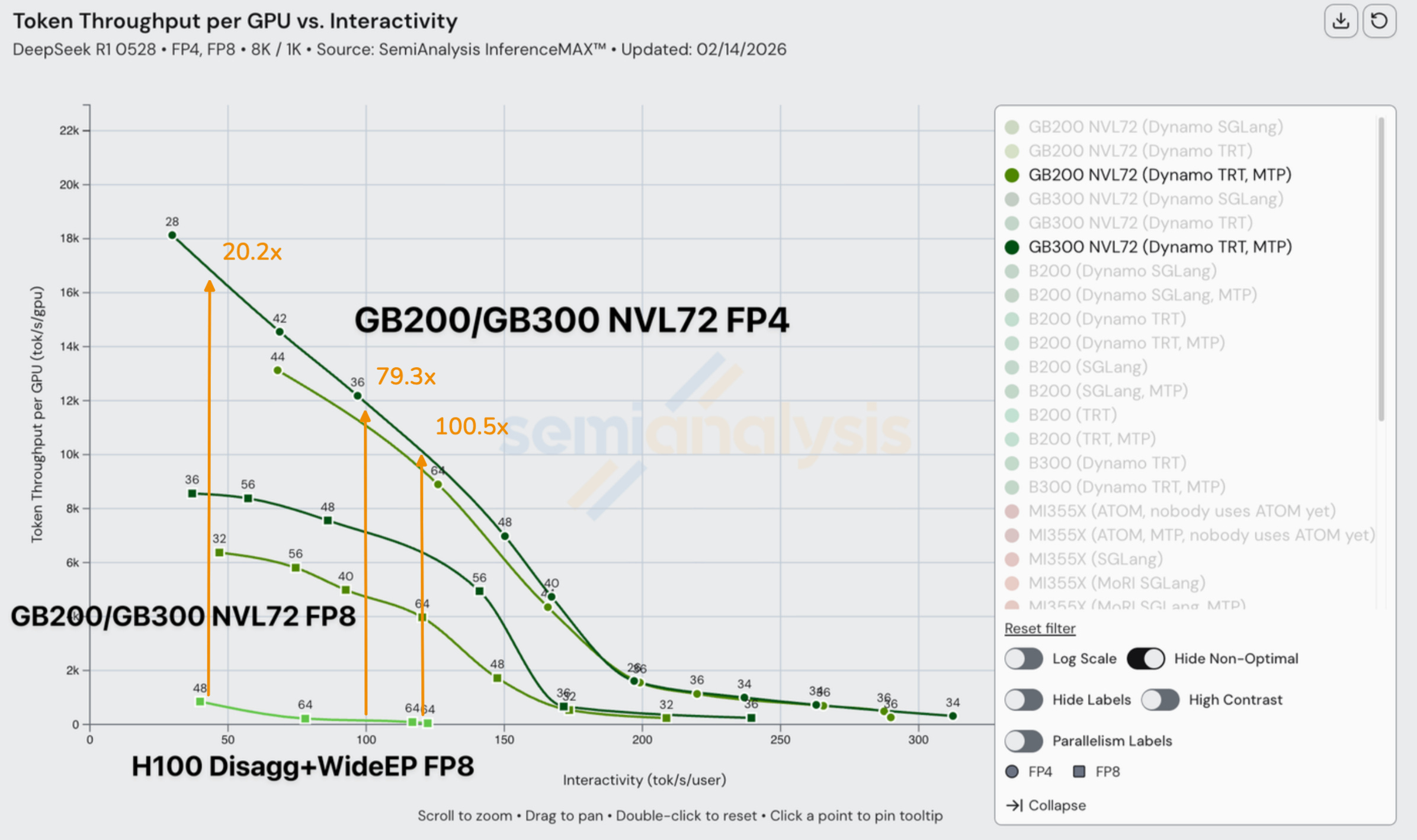
Nvidia’s GB300 NVL72 doesn’t disappoint. It achieves up to 100x on FP8 vs FP4 compared to even a strong H100 disagg+wideEP+MTP baseline and 65x on FP8 vs FP8. On H100 vs GB200 NVL72, we see up to 55x realized performance difference at 75 tok/s/user. Rack scale Blackwell NVL72 is framemogging hopper and makes hopper looks like it is jestermaxxing. As Jensen said at GTC 2025, he is chief revenue destroyer.
At GTC 2024, Jensen claimed that Blackwell will deliver up to 30x perf on inference compared to H100, Jensen under promised & overdelivered on Blackwell inference performance. This should curtail the instances of analysts cracking “Jensen Math” jokes for some time.
Acknowledgments and InferenceX™ (formerly InferenceMAX) Initiative Supporters
We would like to thank Jensen Huang and Ian Buck for supporting this open-source effort by providing access to the latest GB300 NVL72 systems along with access to servers representing all GPU SKUs that they have produced for the past four years. We would like to thank the Nvidia team for allowing us to conduct independent benchmarks across this close to 1000 GPUs. Thank you to Jatin Gangani, Kedar Potdar, Sridhar Ramaswamy, Ishan Dhanani, Sahithi Chigurupati, along with many other Nvidia inference engineers for helping to validate and optimize Blackwell & Hopper configurations.
We’re also grateful to Lisa Su and Anush Elangovan for their support of InferenceMAX and for supporting our work with the dozens of AMD engineers like Chun, Andy, Bill, Ramine, Theresa, Parth, etc that contributed to InferenceMAX & upstream vLLM/SGLang bug fixes, as well as for their responsiveness on helping debug and triage AMD exclusive bugs so as to help optimize AMD performance.
We also want to recognize the SGLang, vLLM, and TensorRT-LLM maintainers for building a world-class software stack and open sourcing it to the entire world. You can check their articles on InferenceX here:
SemiAnalysis InferenceMAX: vLLM maintainers & NVIDIA accelerate Blackwell Inference
SGLang & NVIDIA Accelerating SemiAnalysis InferenceMAX & GB200 Together
The InferenceX initiative is also supported by many major buyers of compute and prominent members of the ML community including those from OpenAI, Microsoft, vLLM, Tri Dao, PyTorch Foundation, Oracle and more. You can find the full list here.
A Primer on Important Technical Concepts
In this section, we will give a brief primer on technical concepts that may help the reader better interpret results. Some readers may not need this and can skip directly to our analysis of results. We will take a deeper dive into some of these topics after the results analysis.
Interactivity vs Throughput Tradeoff
The fundamental tradeoff with LLM inference is throughput versus latency. Interactivity (tok/s/user) describes how fast each user of a system receives tokens – it is the inverse of time per output token (TPOT). Throughput (tok/s) describes how many total tokens a system can crank out across all users. One can achieve higher total throughput by batching requests, but each request will be allocated less FLOPs and thus complete slower. This is analogous to the choice of riding a metro bus vs a race car. The metro bus serves many riders, but also makes frequent stops which takes time, but the cost of the metro bus can be amortized across many passengers. The race car can only carry one or two passengers, but it will make few if any additional stops meaning a faster travel time overall, but it is much more expensive to ride per passenger. The metro bus might make more sense for people heading to the park on a weekend, while the race car might be better for bringing a celebrity to their destination. There is no one size fits all solution.
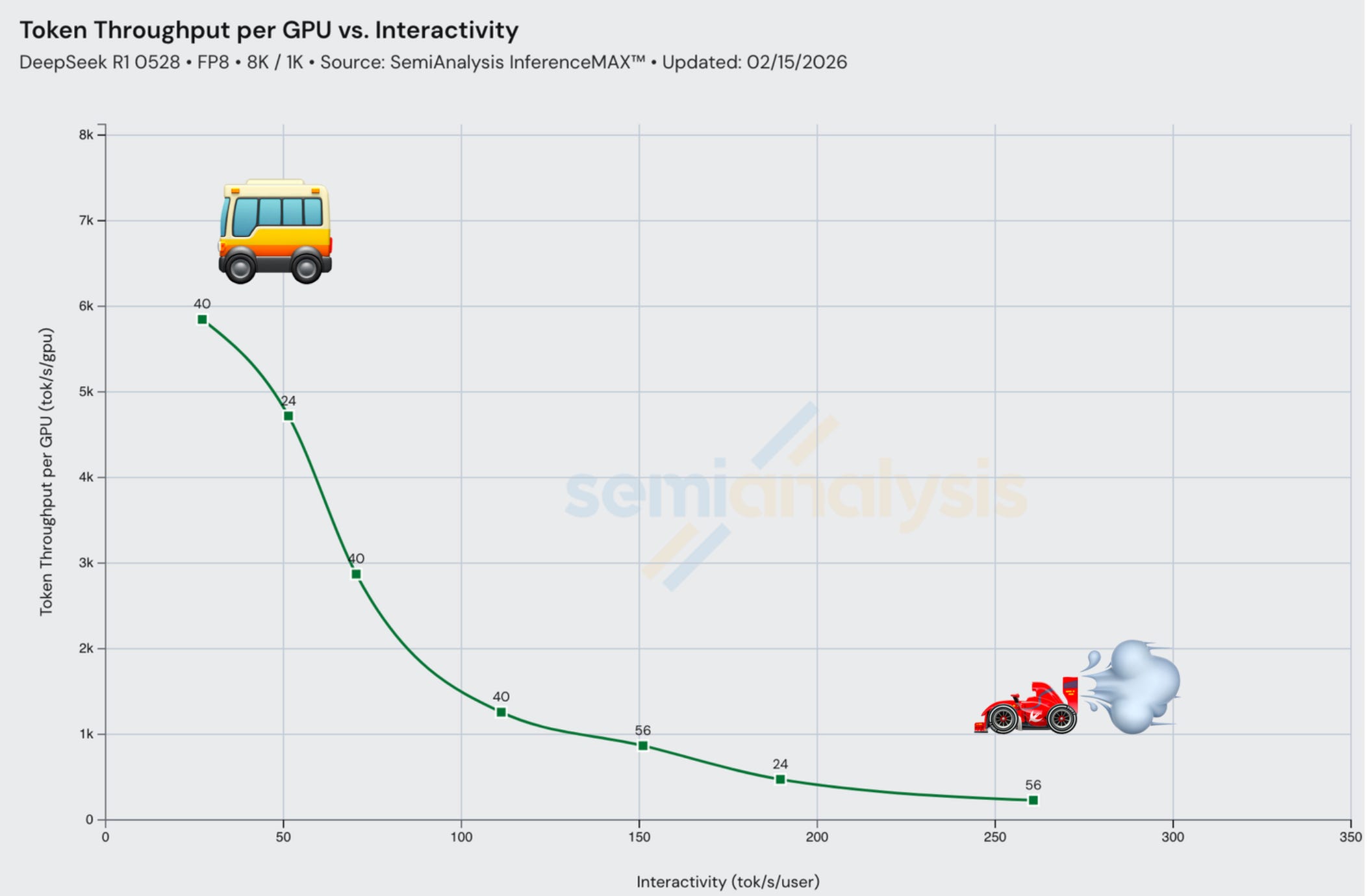
Most benchmark results we will show in this article are InferenceX is a curve. It is important to analyze throughput at various levels of interactivity/latency instead of just looking at maximum achieved throughput (which normally can only be achieved at a single low interactivity). With inference, there is no one size fits all use case. The level of interactivity and throughput needed depends on the use case. For instance, real-time speech models require extremely low latency so that the end user can maintain a natural “conversation” with the LLM, whereas a basic QA chatbot may allow for higher latency. We leave it up to the reader to look at the curve and apply this principle to identify where their use case falls on the throughput-interactivity curve.
The Cost/Perf per TCO vs Interactivity/End-to-End Latency curve mostly follows the Throughput vs Interactivity/End-to-End Latency Curve: More tokens/hour leads to a lower cost per token as fixed $/hour costs are amortized over more tokens produced.
Prefill and Decode Phases
Inference contains two main phases: prefill and decode. Prefill occurs during the first forward pass of a request’s lifetime. It is computationally intensive since all tokens in the request are processed in parallel. This phase is responsible for “filling up” the KV cache for a sequence. After prefill, responses are generated (or decoded) one token at a time. Each forward pass loads the entire KV cache for a sequence from HBM, while only performing the computation for a single token, making decode memory (bandwidth) intensive.
When prefill and decode performed on the same engine, prefill constantly disrupts decode batches leading to worse overall performance.
Disaggregated Prefill
Disaggregated prefill (aka PD disaggregation or simply “disagg”) is the practice of separating the prefill and decode phases across separate pools of GPUs or clusters. These separate prefill and decode pools can be tuned independently and scaled to match the needs of workloads.
Tensor Parallel, Expert Parallel, Data Parallel (TP, EP, DP)
TP allows for maximize interactivity at small batch sizes, but it must carry out an all-reduce at every layer. EP shards experts, exploiting MoE sparsity, with the drawback being an all-to-all collective (which is more costly than simpler collectives like all-reduce) is carried out for MoE layers and can be imbalanced at small batches. DP replicates the entire model (or just parts of a model, like attention) on multiple groups of GPUs (ranks) and then load balances requests among ranks. It is the simplest to scale, but repeats weight loading which can be wasteful at scale.
Tracking Improvements Over Time
One of the main goals of InferenceX is to visualize performance improvements over time. While new chips are released on an O(yearly) cadence, software releases happen on an O(weekly) cadence. Our goal is to constantly update recipes with the latest and greatest software improvements and benchmark the configurations.
DeepSeek R1
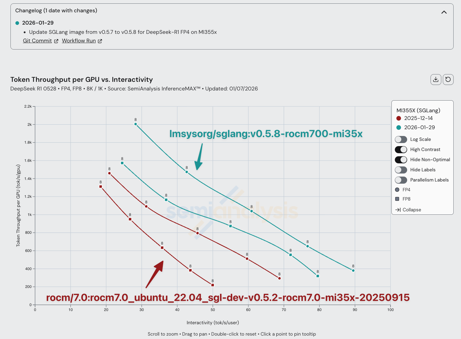
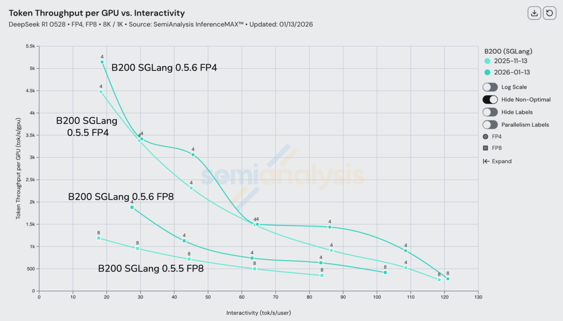
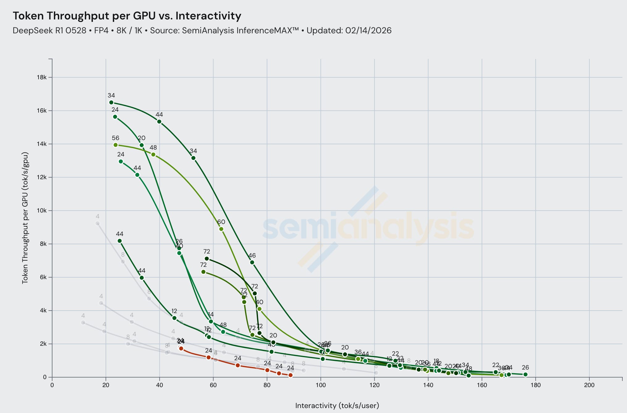
The AMD team has significantly improved performance for all configurations of SGLang DeepSeek R1 FP4. For the same interactivity, AMD has almost doubled the amount of throughput in the span of less than 2 months. Moreover, we have pushed AMD to upstream performance enhancing changes from their forked SGLang images into the official SGLang image. From December 2025 to January 2026, AMD’s software was improved up to 2x in performance.
In order to continue becoming closer to an first class experience, AMD needs increase their support of vLLM & SGLang maintainers through compute contributions and code contributions & having more reviewers that work for AMD to speed up the review process of AMD PRs into the upstream.

On the other hand, Nvidia’s results were more consistent, with minor improvements for B200 SGLang over a similar time period.
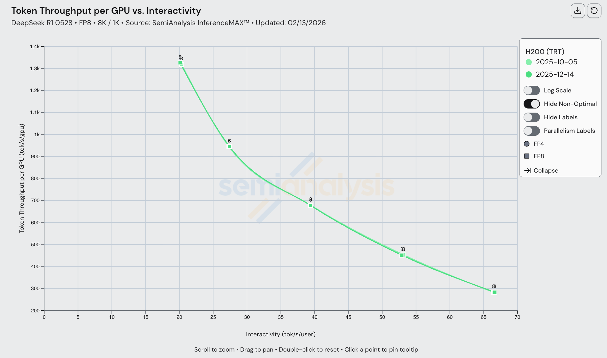
Many of the mature SKUs had minimal improvements. For example, H200 TRT single node has not changed in performance in the span of 4 months since October, but this is because Hopper support has been excellent since day 1, and performance has close to peak theoretical for this workload all along, making it hard to deliver incremental performance gains.
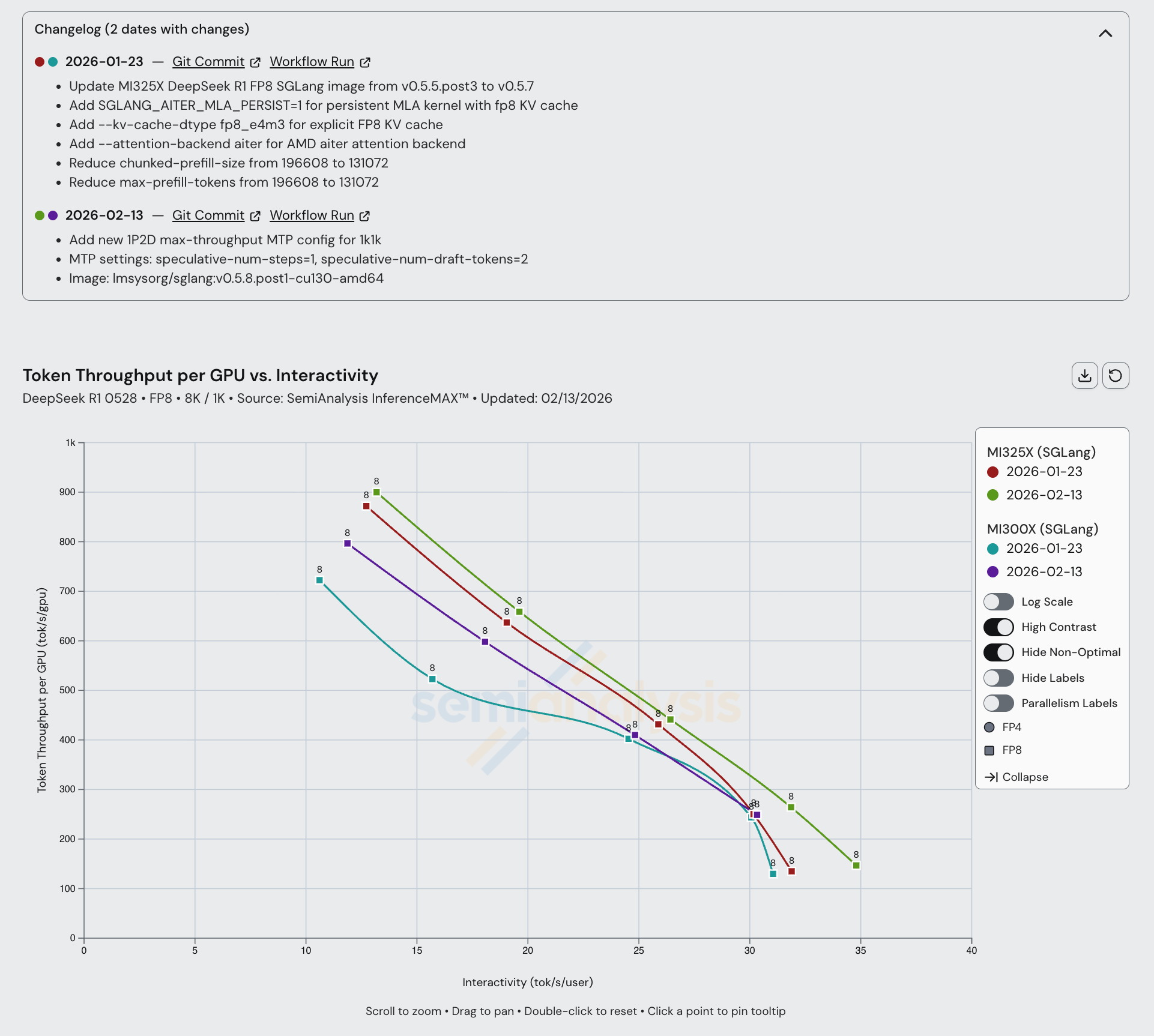
MI300X and MI325X have seen some improvements, mainly from the most recent SGLang release. Note that for much of the history of InferenceX, AMD was using “private” ROCm images that were not upstreamed, so runs prior to ~Jan 2026 cannot be compared directly to those that are more recent.
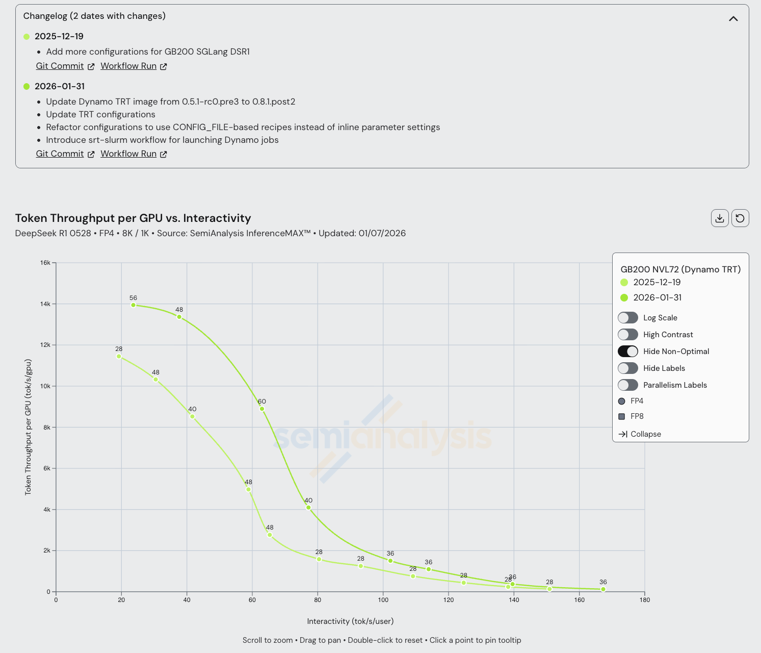
GB200 Dynamo TRT-LLM disagg has seen some significant improvements as well, with a 20% increase in max throughput in the span of a little over 1 month. We also see improvements in the middle interactivities, where wide EP is deployed. This is likely due to maturing wide EP kernels on GB200.
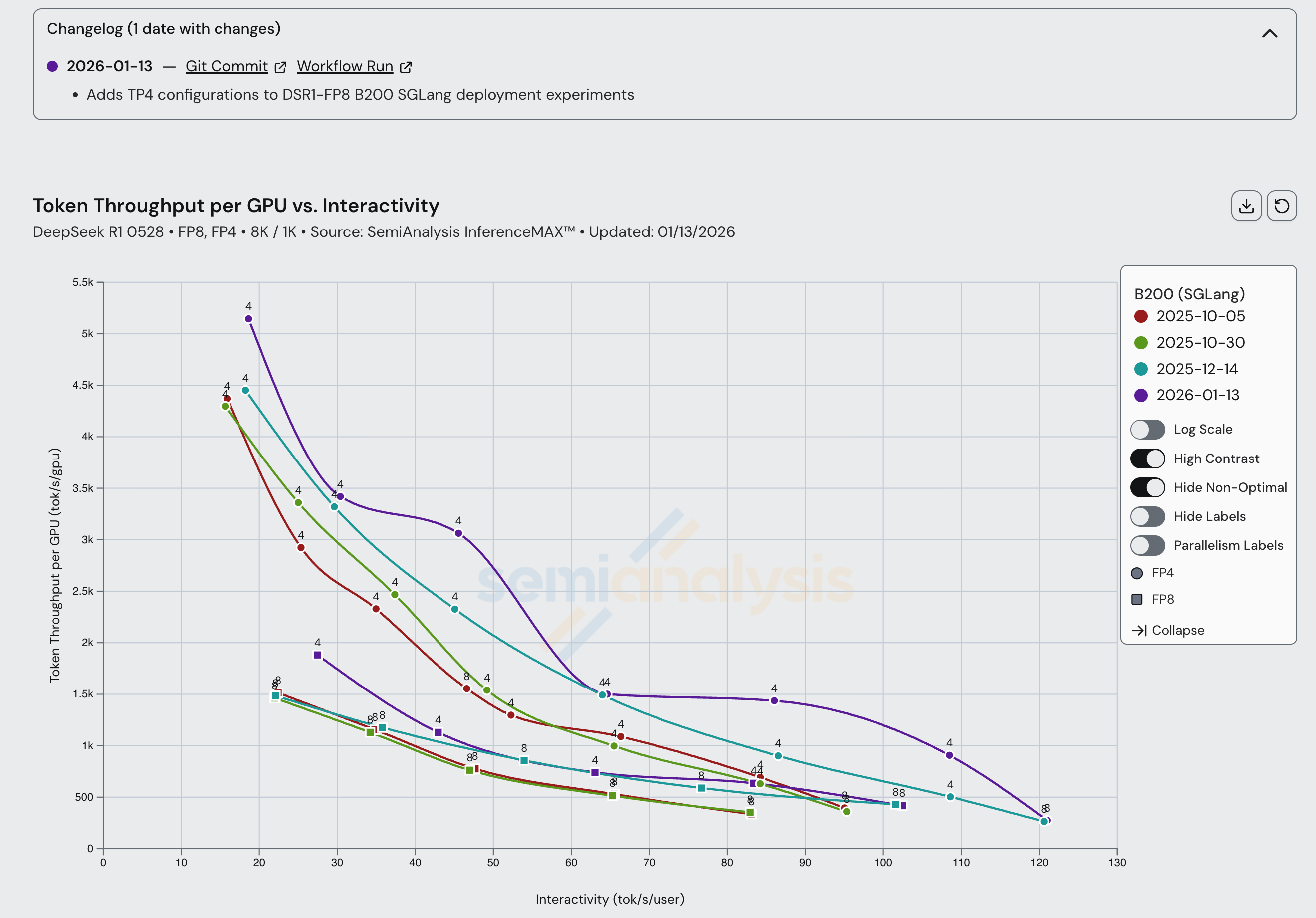
B200 SGLang has seen steady and continuous improvement for both FP4 and FP8 scenarios since our initial launch, with throughput per GPU doubling at some interactivity levels since last October.
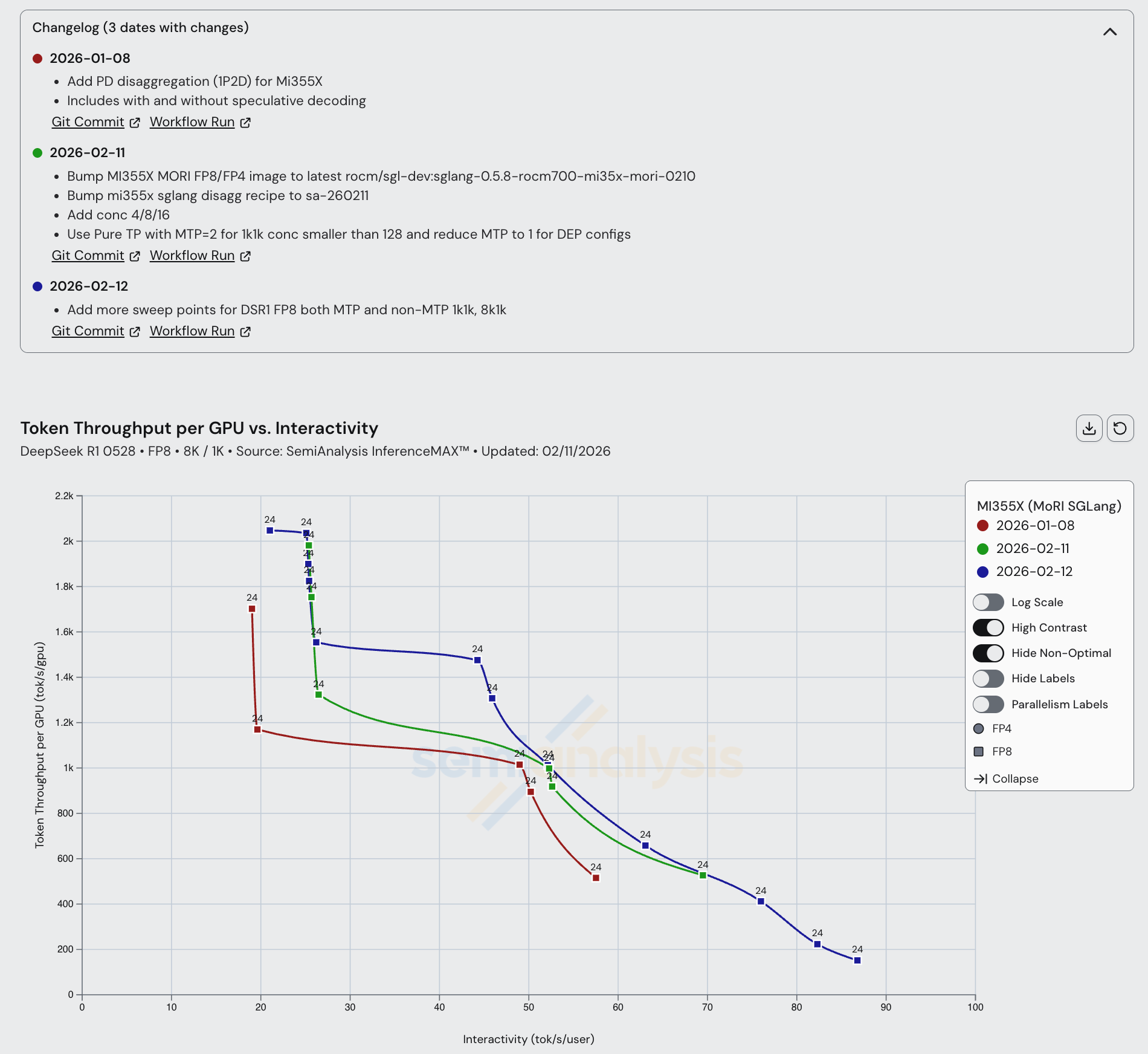
For MI355X Disaggregated inference serving, AMD recommends using SGLang with MoRI. MoRI is AMD’s MoE dispatch/combine collective and KV Cache transfer library built from first principles by AMD’s cracked 10x China-based engineering team. Although MoRI needs much more open CI and testing, we are strong supporters of the direction that MoRI is taking. This is because instead of taking AMD’s historical approach, which was to fork NVIDIA’s NCCL into RCCL, MoRI is built from scratch by taking the lessons from RCCL/NCCL and building an entirely new package from first principles. The use of MoRI has also delivered good speedups in the span of more than a month, with throughput per GPU increasing by more than 20% in the 20-45 tok/s/user interactivity range.
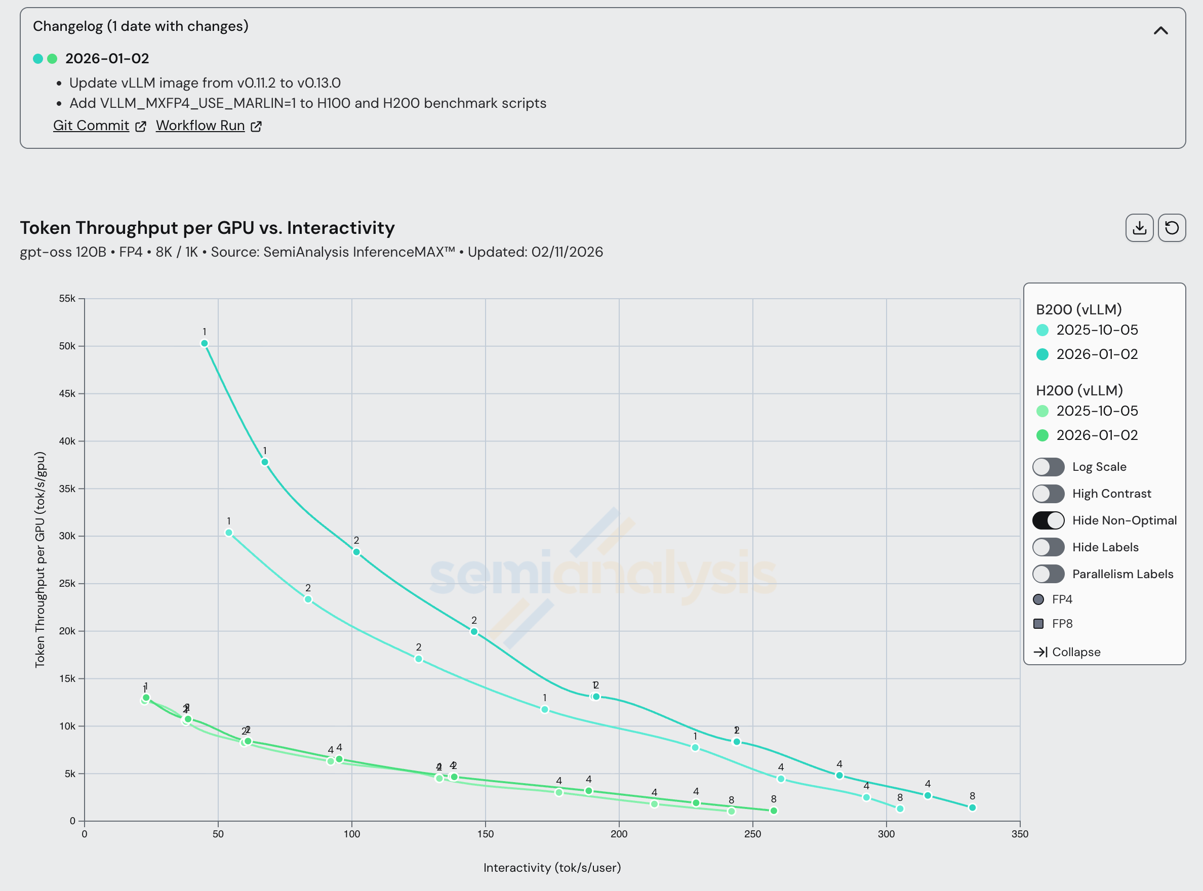
GPT-OSS 120B
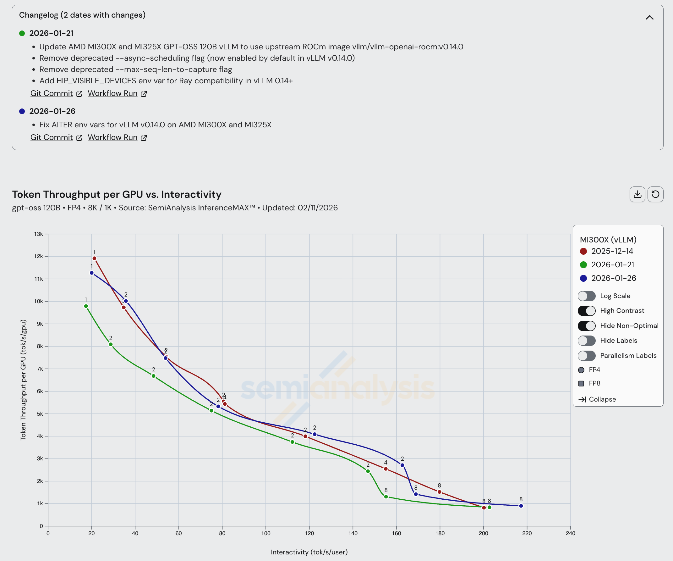
For MI300X and MI325X, we have seen marginal improvements across the board. Some AITER optimizations helped MI300X performance across all interactivities, and switching to the upstream vLLM ROCm image led to improvements.
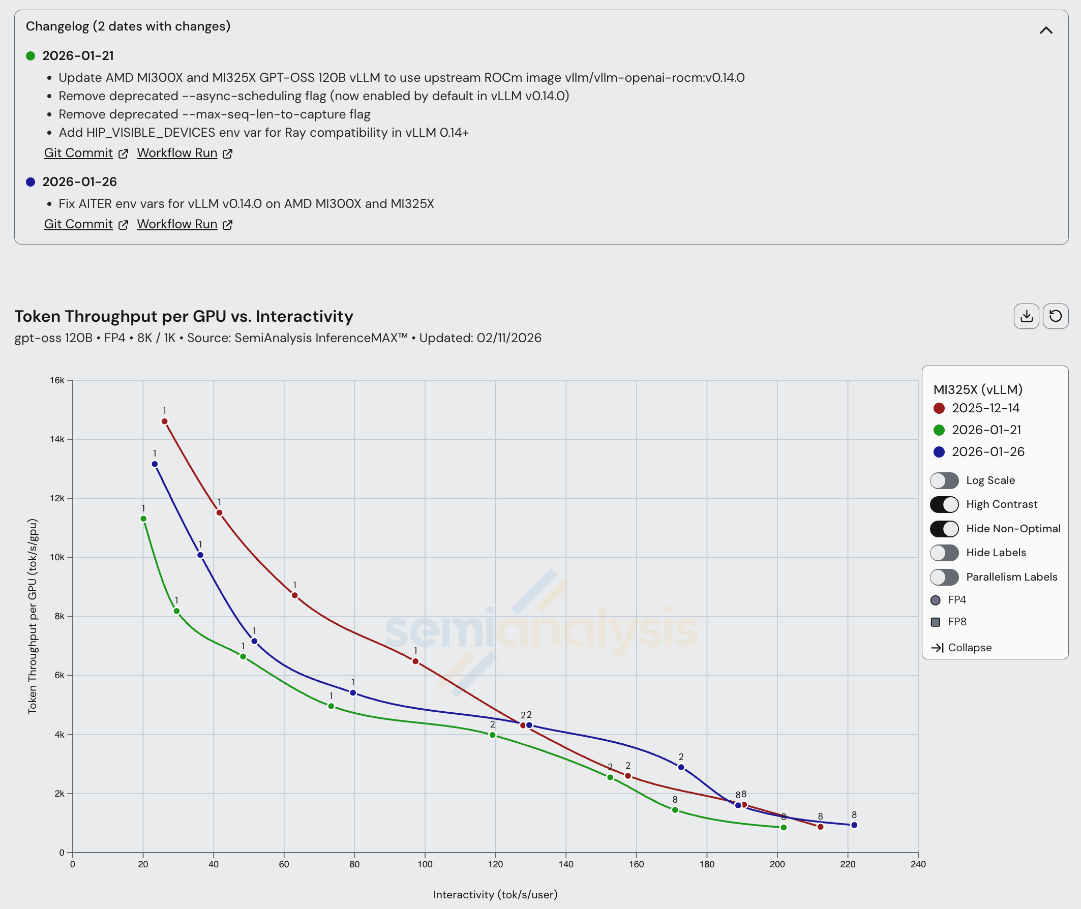
In the case of the MI325X, it appears that not all performance enhancements that were present in the downstream ROCm fork image (used during the October 5th, 2025 run) have made it into the official vLLM ROCm image.
Unfortunately, the MI355X literally still uses a fork of the vLLM 0.10.1 build rocm/7.0:rocm7.0_ubuntu_22.04_vllm_0.10.1_instinct_20250927_rc1). We would love to have seen it updated it by now, but unfortunately the current official image (0.15.1, at the time this article was written) is not yet optimized for the MI355X and runs into hard errors. We had also run into hard errors crashes on Mi355 for vLLM 0.14. Word on the street is that vLLM 0.16.0 will finally deliver all the changes needed for better MI355X performance.
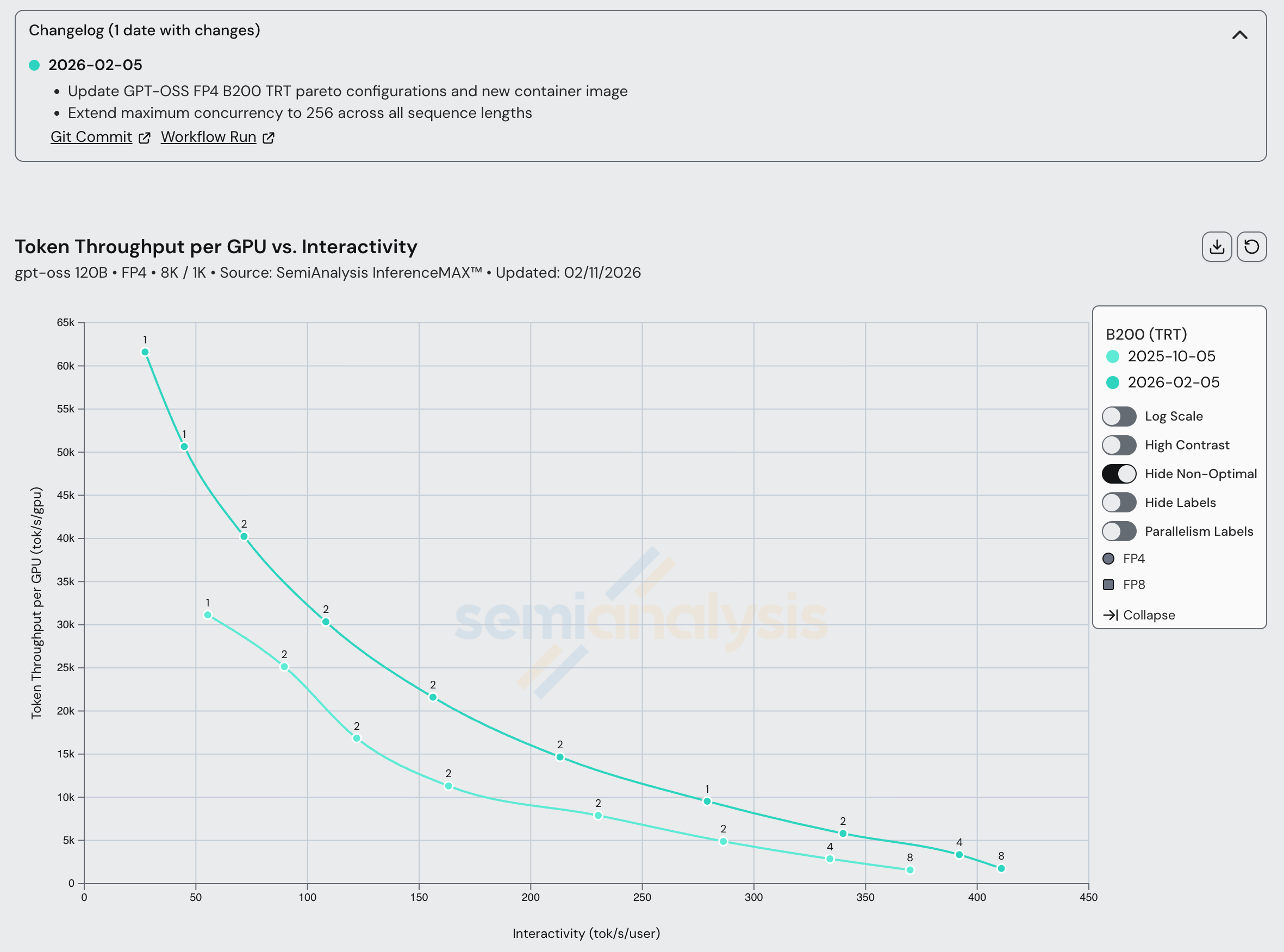
Turning back to Nvidia’s systems, both Hopper and Blackwell saw a steady performance increase between vLLM 0.11.2 and 0.13.0. Soon, we will update recipes for Nvidia GPUs to use the latest vLLM version and we expect even greater performance gains after making the switch. We also observed a performance bump in the latest 1.2.0 version of TRT-LLM.
Disaggregated Inference Frameworks
NVIDIA uses Dynamo for its disaggregated inference setup. Dynamo is an inference framework designed for multi-node distributed inference, featuring techniques such as prefill-decode disaggregation, request routing, and KV cache offloading. It is inference-engine agnostic, allowing us to use SGLang and TRT LLM as backends in our benchmark. For AMD, we use SGLang with two different KV cache transfer frameworks: MoRI and Mooncake. MoRI is a high-performance communication interface focusing on RDMA and GPU integration, offering applications such as network collective operations and expert parallel kernels. Mooncake, which recently joined the PyTorch ecosystem, supports prefill-decode disaggregation and many fault tolerant multi-node features.
DeepSeek Disagg +WideEP Results Deep Dive
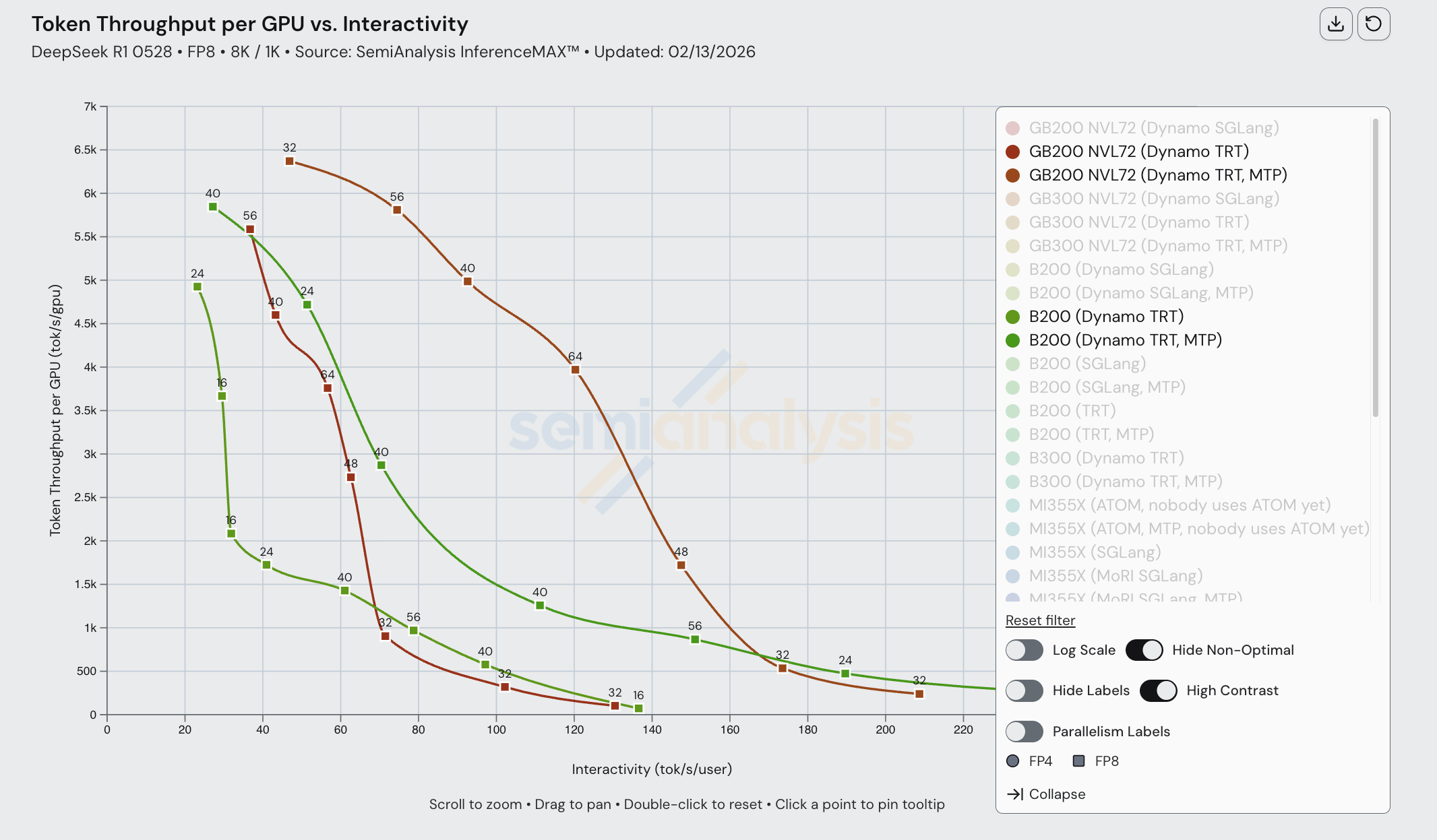
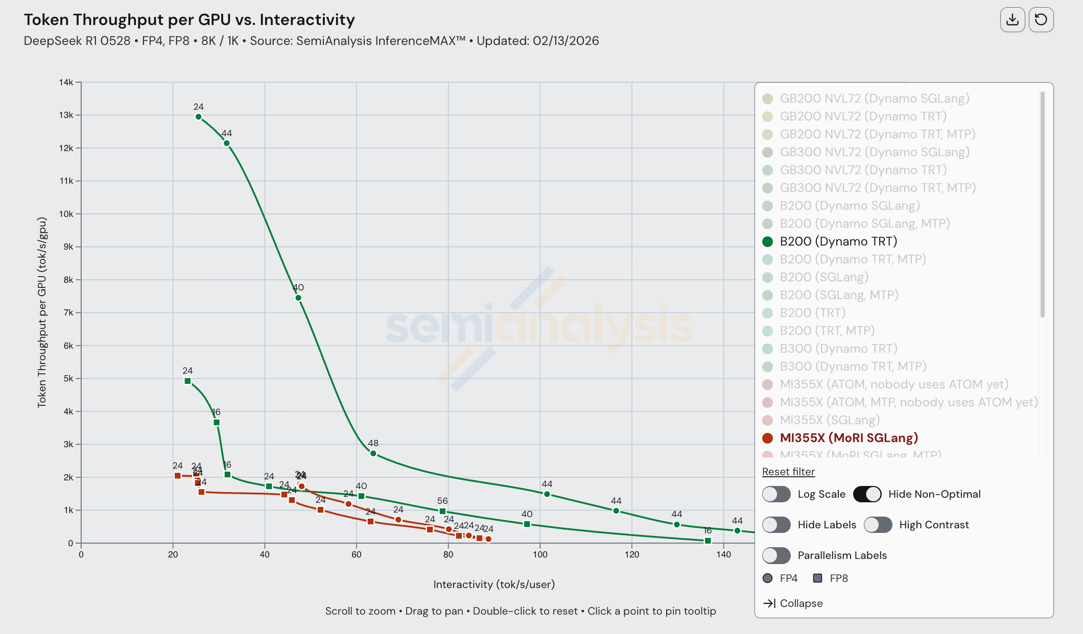
At almost all interactivity levels, disagg outperform aggregated inference (grey lines) in terms of total token throughput per GPU. Multi-node disaggregrated prefill framemogs single node aggregrated serving.
Nvidia continues to push new updates for B200/GB200 FP8. The latest data on DeepSeek FP8 B200 TRT single node (both MTP enabled/disabled) vs GB200 Dynamo+TRT disagg (both MTP enabled/disabled). This indicates consistent engineering effort to improve rack-scale inference software and wideEP kernels.
When comparing MI355X disaggregated inference vs aggregated inference, we noticed a similar pattern. Disaggregated inference only overtakes aggregated inference at low interactivity, high batch sizes. This is true across FP4, and it is likely due to poorly optimized kernels.
When composing disagg prefill+wideEP with FP4 on the MI355X, we observe suffers subpar performance.
Although theoretical modeling shows that disagg inference on MI355Xs should perform way better than single node, disagg actually performs worse for higher interactivity levels due to a lack of kernel and collective optimization in the ROCm software stack when composing multiple SOTA inference optimizations together.
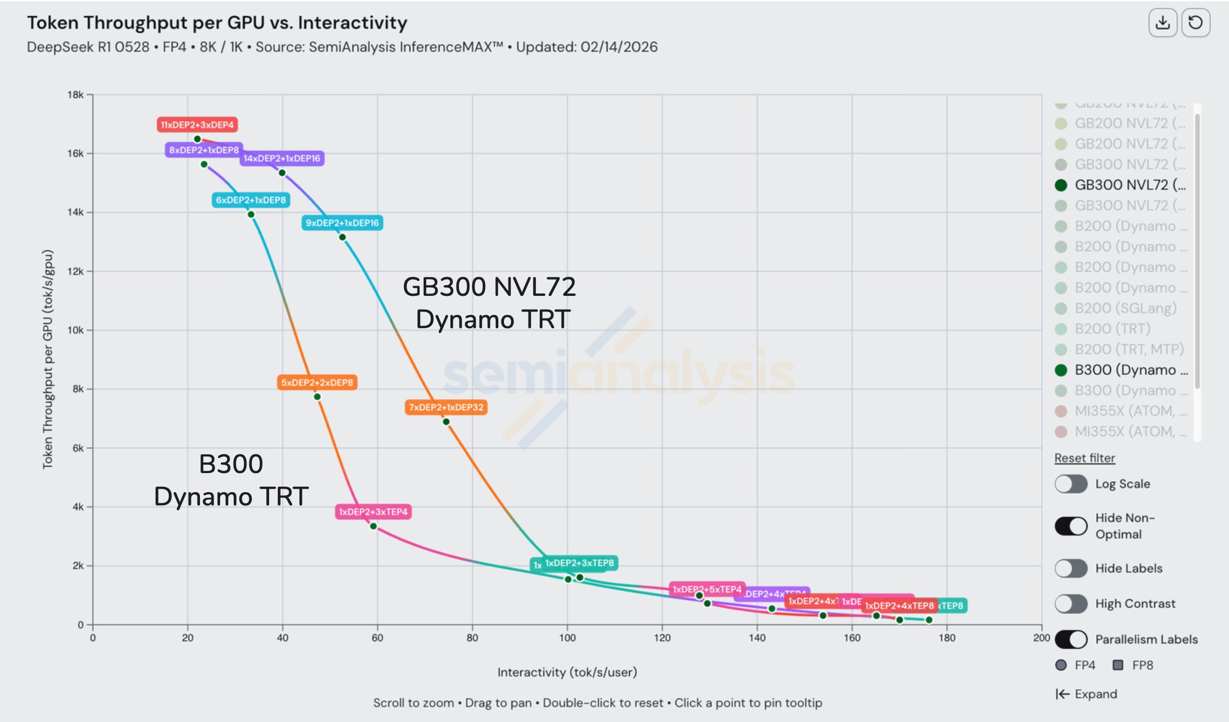
Nvidia TensorRT LLM and NVL72
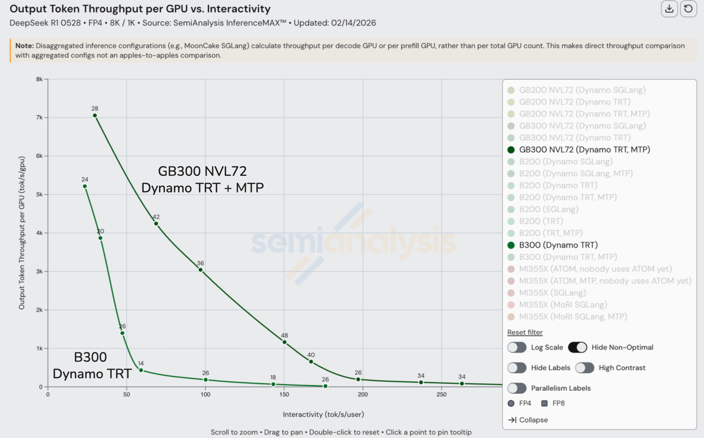
TensorRT LLM already serves billions of tokens per hour globally across providers like TogetherAI and other advanced providers, and it has really allowed the GB200 NVL72 and GB300 NVL72 to shine, delivering more than double the performance at high throughput. MTP boosts these results even further, making use of the chips’ full potential.


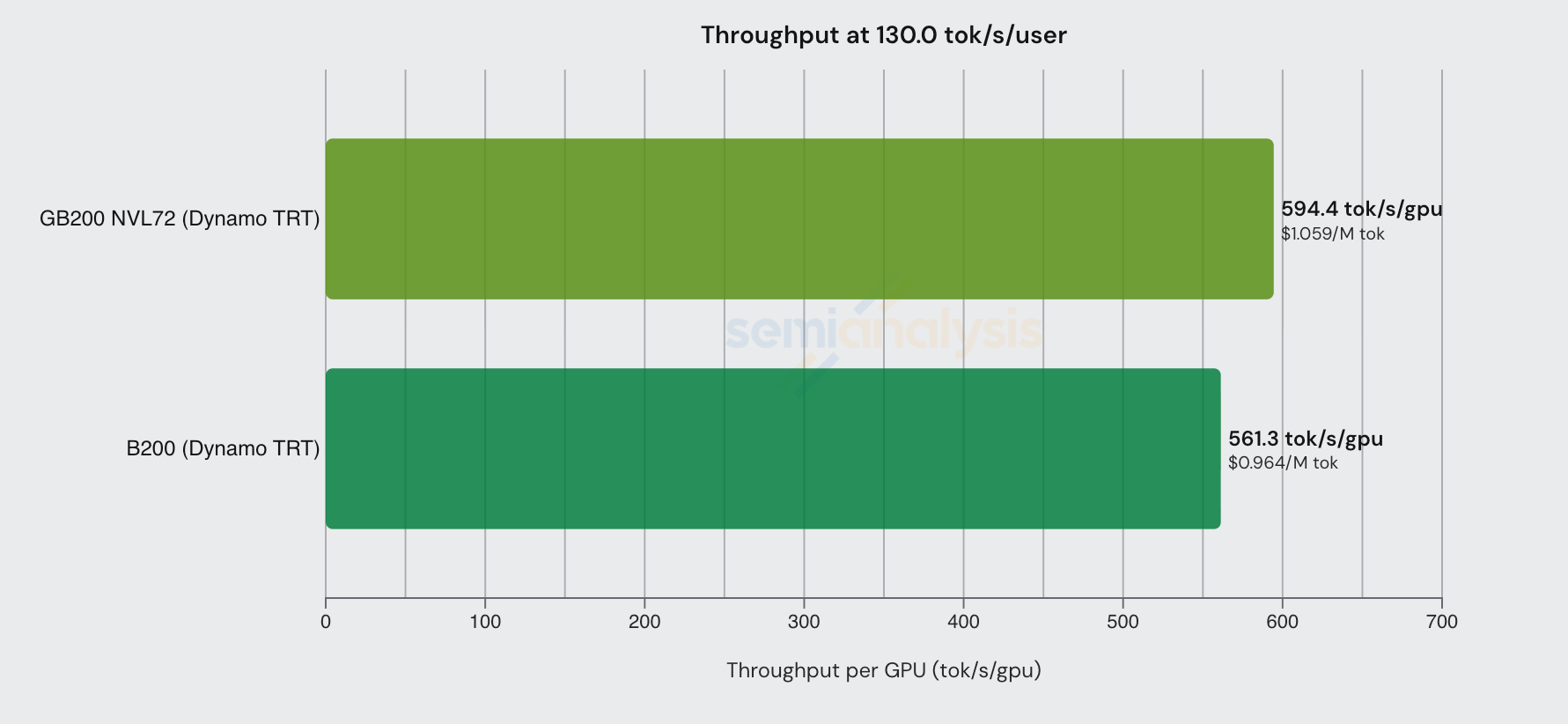
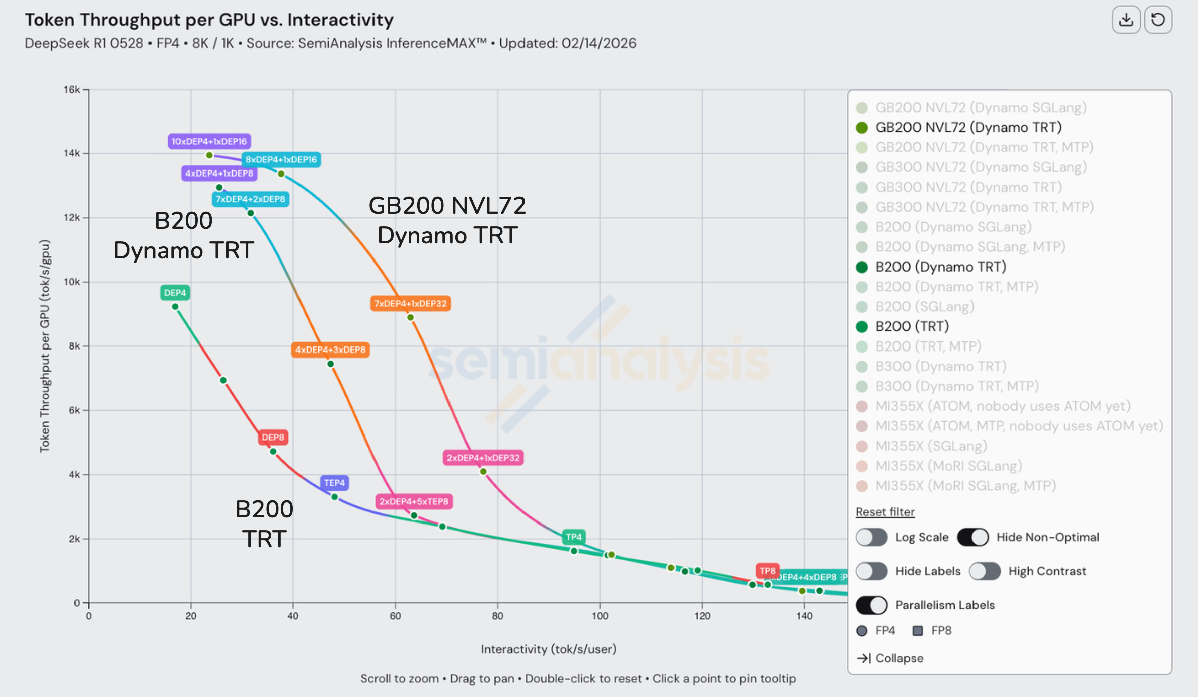
The benefits delivered from the larger world size of the NVL72 family is also evident if we look at cost graphs. At a fixed interactivity level of 60 tok/s/user, each GB200 NVL GPU produces slightly less than triple the number of tokens/s than each B200 does.
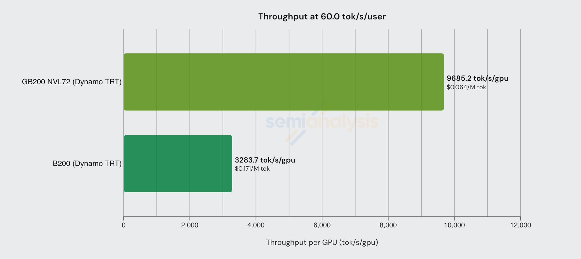
This gap shrinks as interactivity increases. At 130 tok/s/user, the GB200 NVL72 has nearly no advantage and is even more expensive on a $/Million tokens basis. At low batch sizes, the inference workload shrinks enough to fit within a single HGX node’s NVLink domain (i.e. 8 GPUs), and the GB200 NVL72’s larger scale-out advantage starts to disappear.
Nvidia versus AMD Disagg Prefill
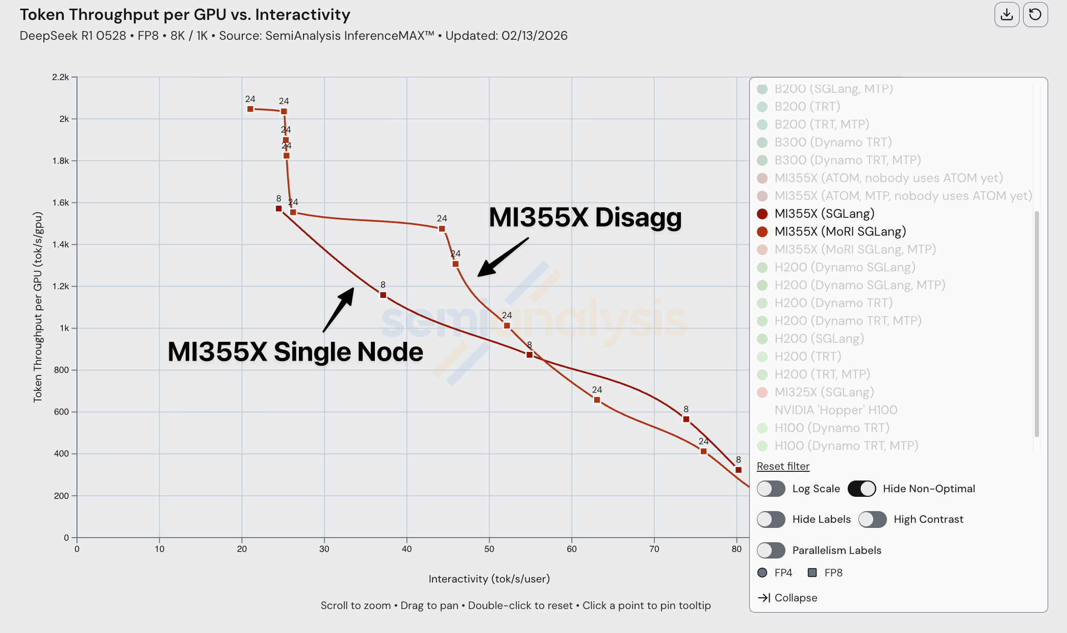
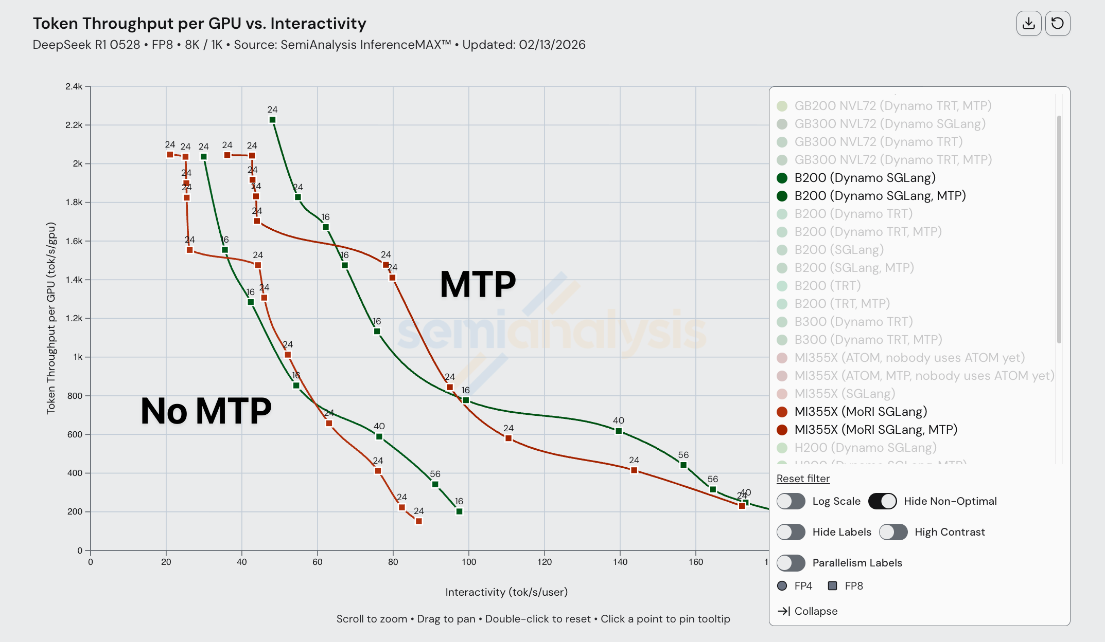
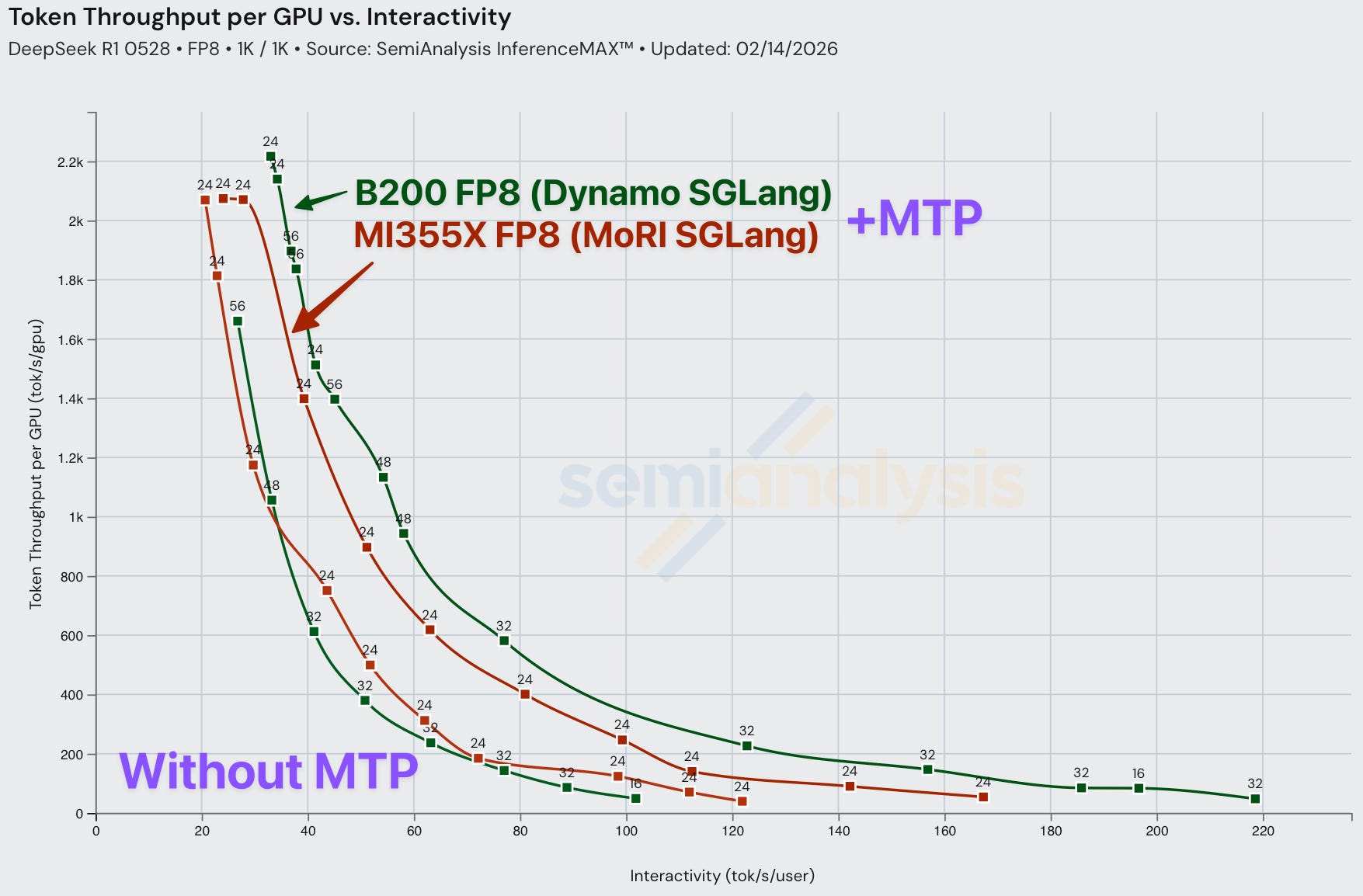
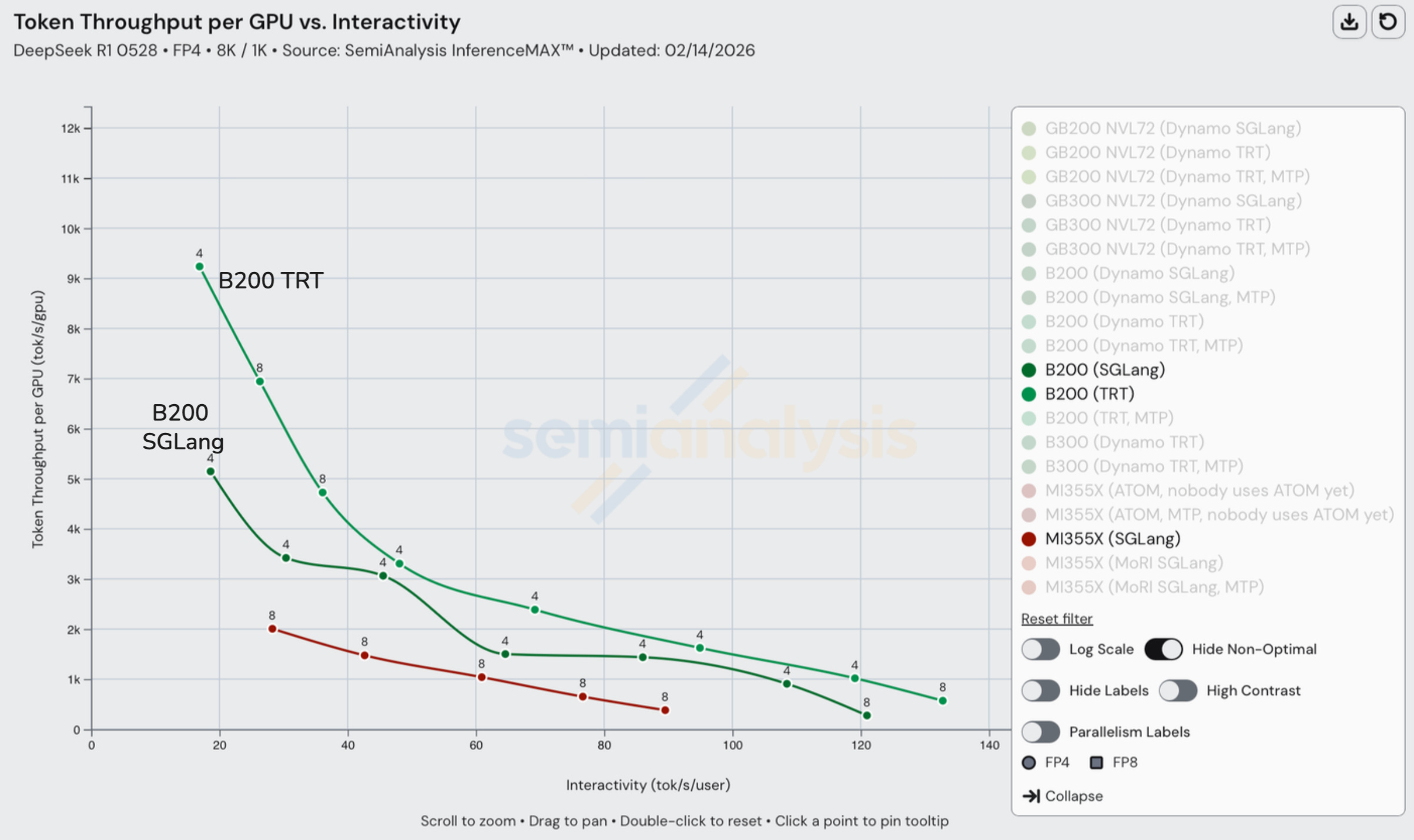
With today’s release of InferenceXv2, for the first time the ML community is able to see a full Pareto frontier for open-source MI355X distributed inference. We show Pareto curves for the B200 and MI355X with and without enabling MTP.
For FP8 disagg prefill, MI355X (MoRI SGLang) is quite competitive with B200 (Dynamo SGLang). Wide EP is not used for either of these configs as all prefill/decode instances run using EP8 at the most. At both ends of the throughput versus interactivity Pareto frontier, MI355X falls behind the B200 slightly. However, MI355X disagg has a slight advantage for certain levels of interactivity in the middle of the curve. Both the B200 and the MI355X benefit from employing MTP, and we observe the same relative performance improvement for both chips when using MTP.
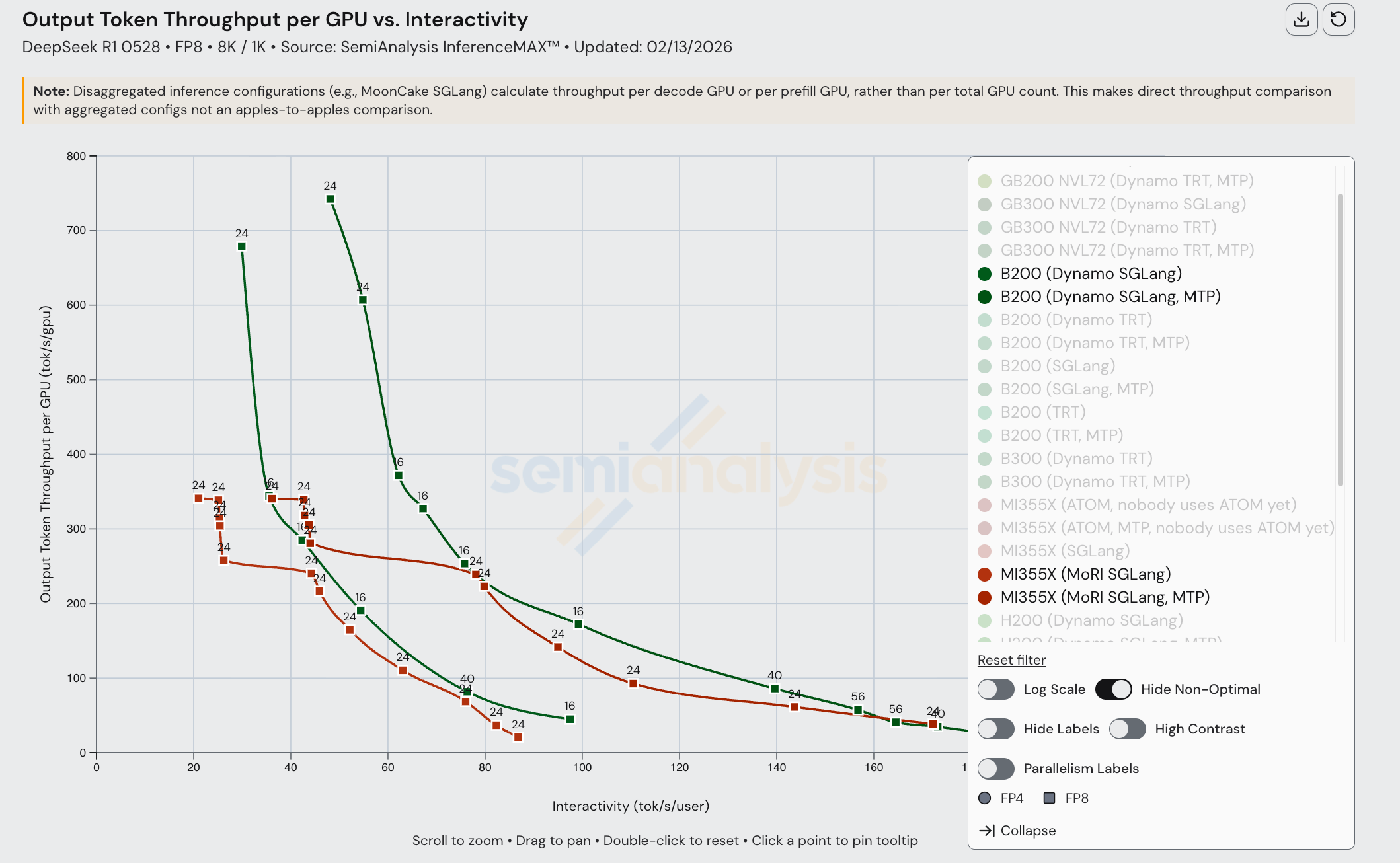
However, if we were to only measure output (decode) token throughput, we see that output token throughput is much higher for the B200 than for the MI355X at lower interactivity levels. Note that when looking at output token only throughput for disaggregated inference configurations, we normalize throughout by the number of decode GPUs, not total GPUs. It is possible that different numbers of GPUs are used for output when running inference jobs on the B200 and MI355X, but the bottom line is that whatever configuration decode is run on, B200 gets the decode job done faster.
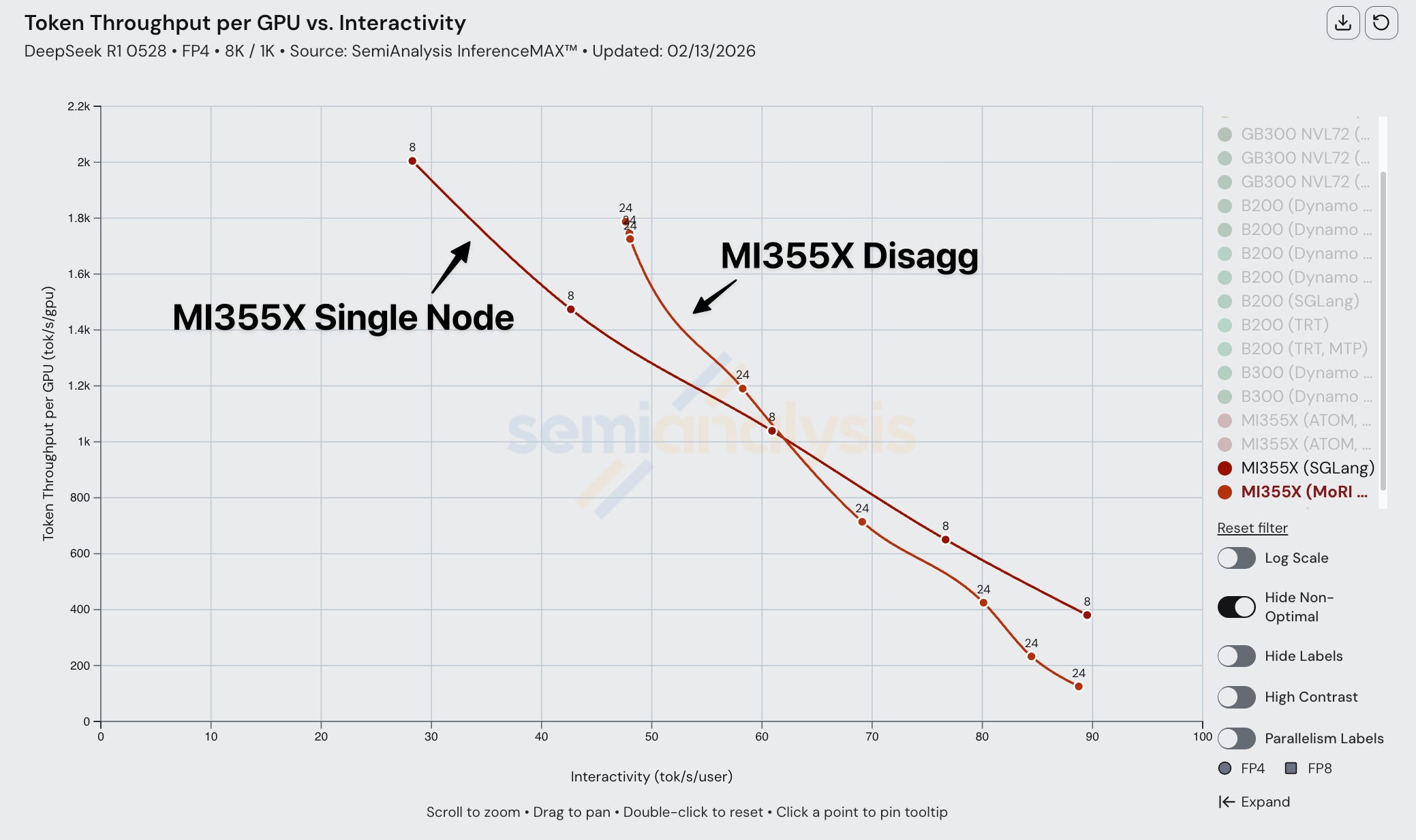
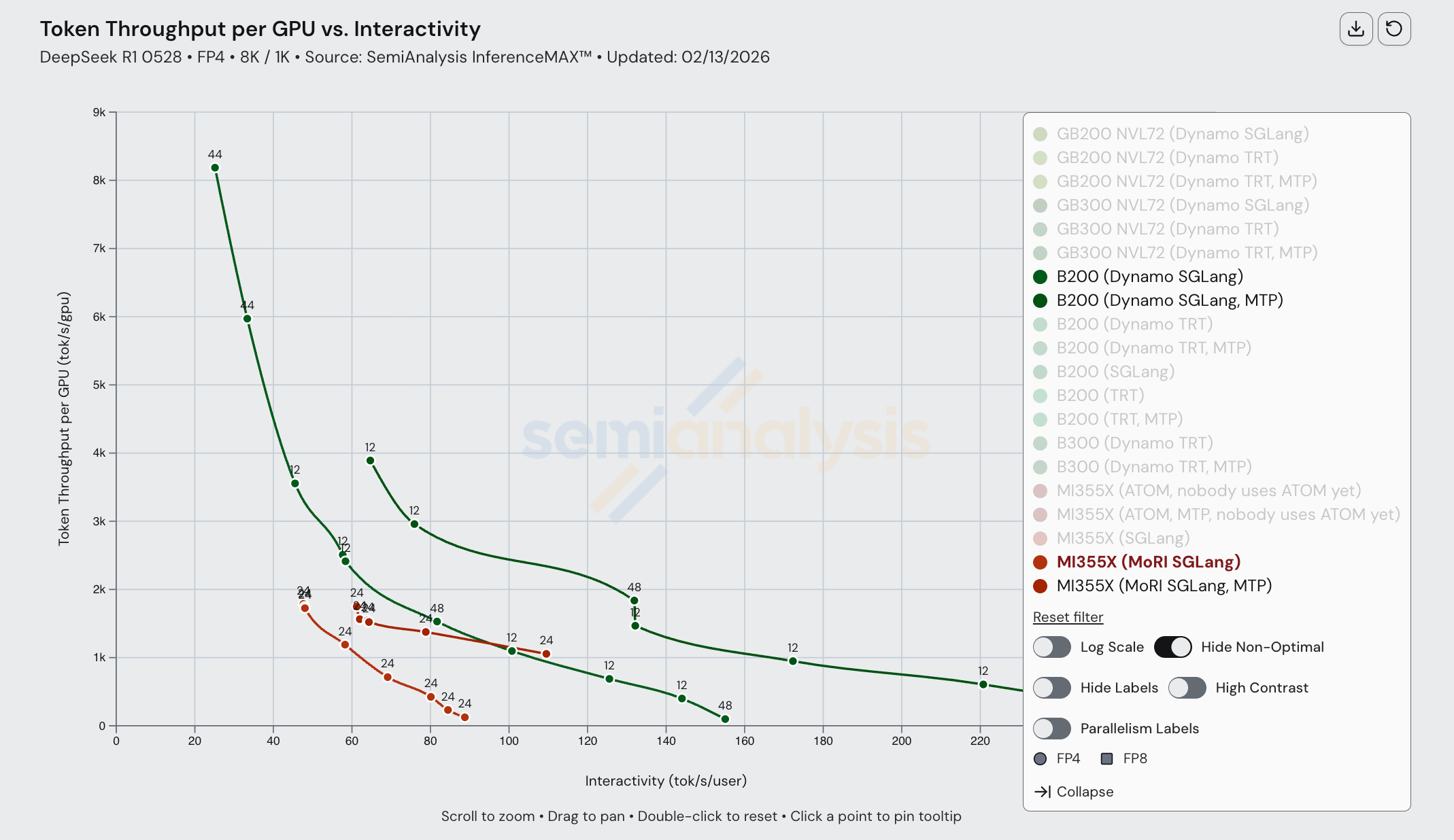
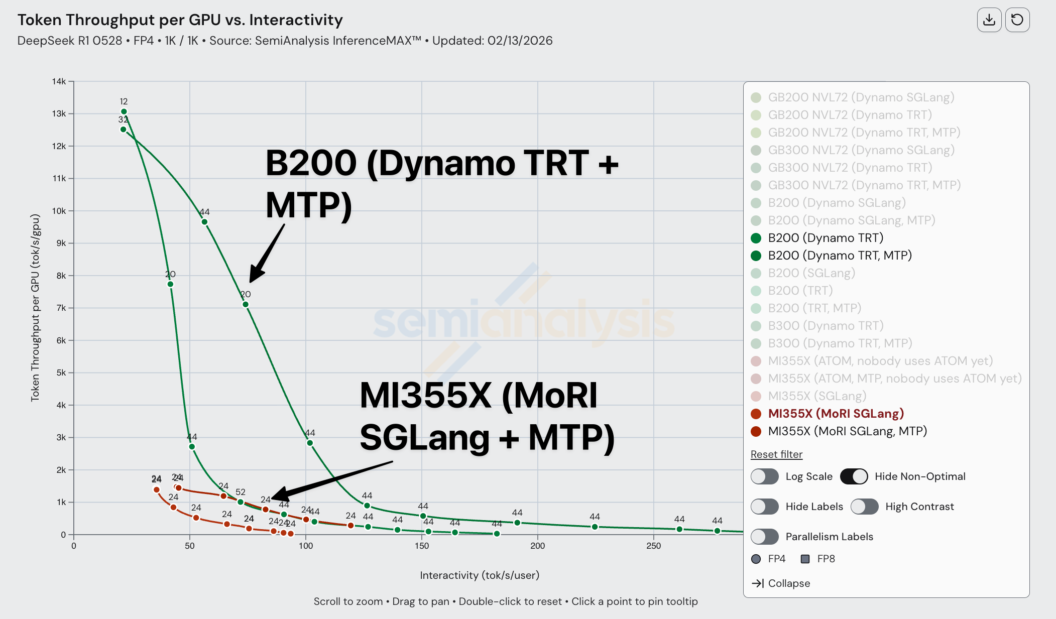
Despite the MI355X being competitive in FP8 disagg, its FP4 performance suffers from composability issues. AMD single node FP4 performance is decent, but when we compare AMD FP4 disagg prefill to Nvidia, performance is subpar and the MI355X gets absolutely mogged by Nvidia’s B200. In a 1k1k scenario, the MI355X (MoRI SGLang) with MTP barely manages to beat the B200 (Dynamo SGLang) without MTP.
Once we bring Dynamo TRT-LLM into the equation, the B200’s performance is boosted even more to the point that the MI355X even with MTP can’t match the B200’s performance with Dynamo TRT-LLM and MTP. The MI355X can only match the B200 (without MTP) in performance by using MTP, and only for a range of interactivities from ~60 tok/s/user through ~120 tok/s/user.
When comparing Dynamo TRTLLM B200 disagg prefill to SGLang MoRI MI355 disagg prefill, AMD gets framemogged due to the more mature implementation of disagg prefill on TRTLLM.
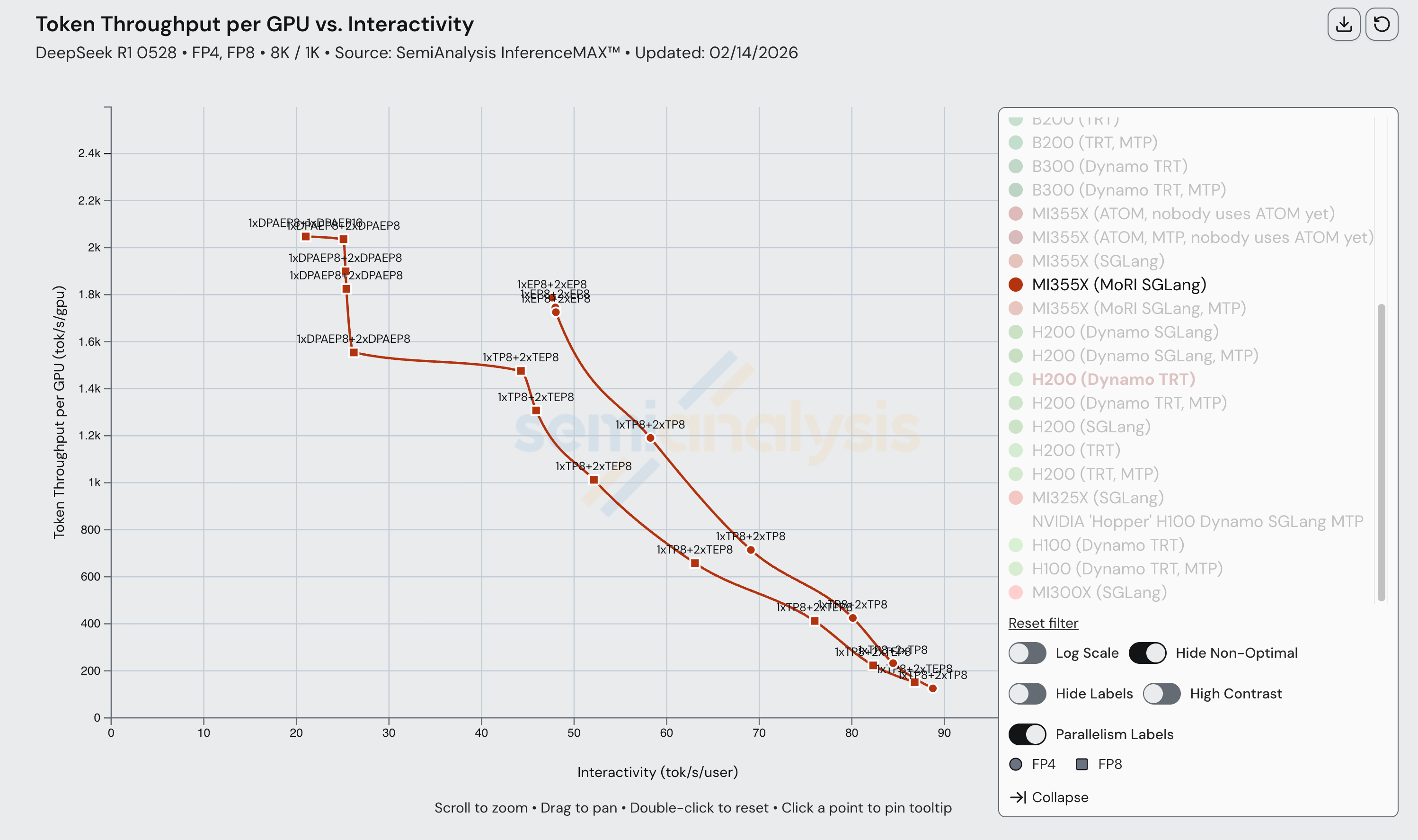
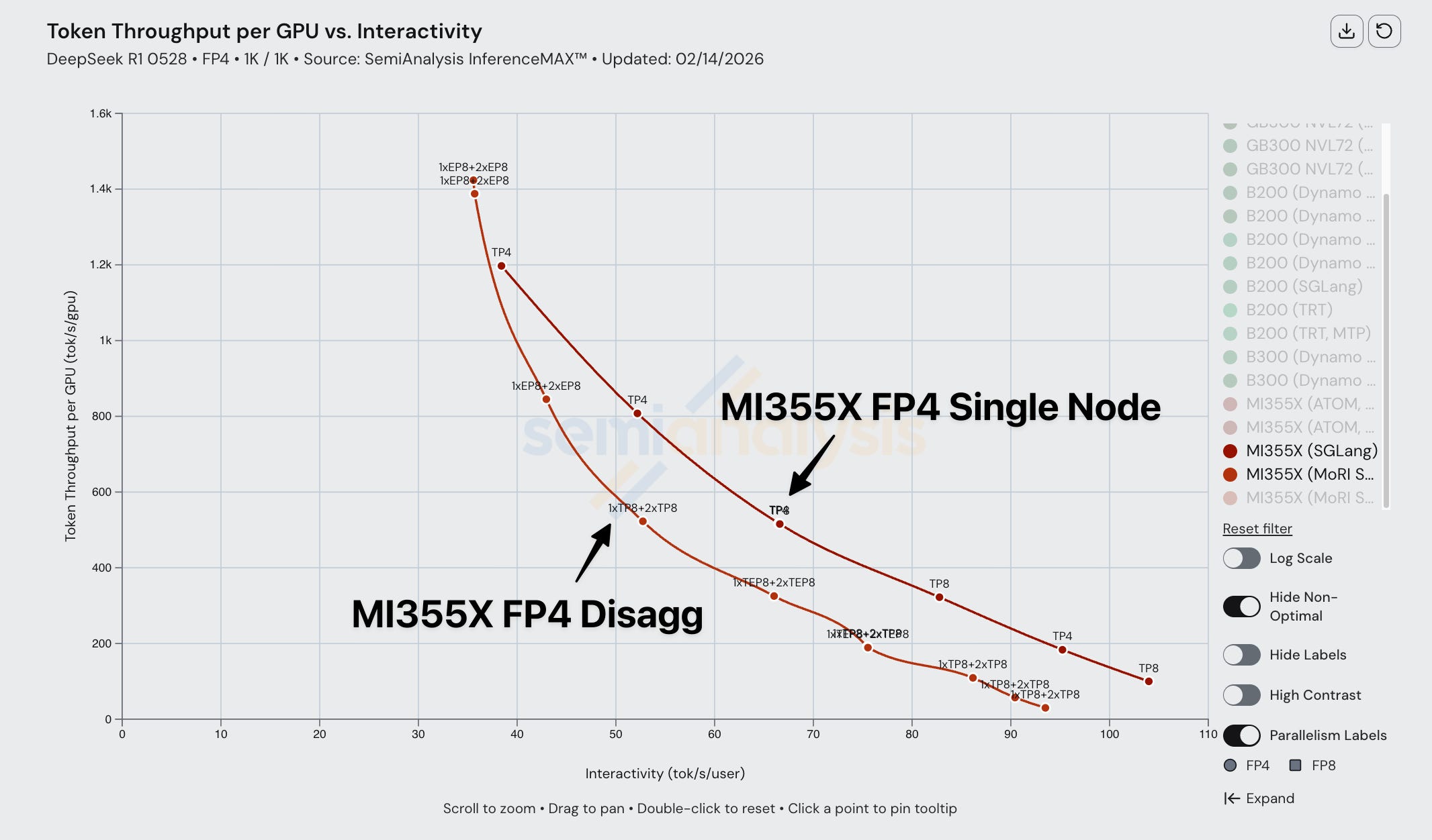
The diagram below shows us the various parallelism configurations that form up the MI355X (MoRI SGLang) Pareto frontier. Note that currently, wide EP is not employed for any points (i.e., configurations with EP 16, 32, etc.).
Unpacking Inference Providers’ Unit Economics
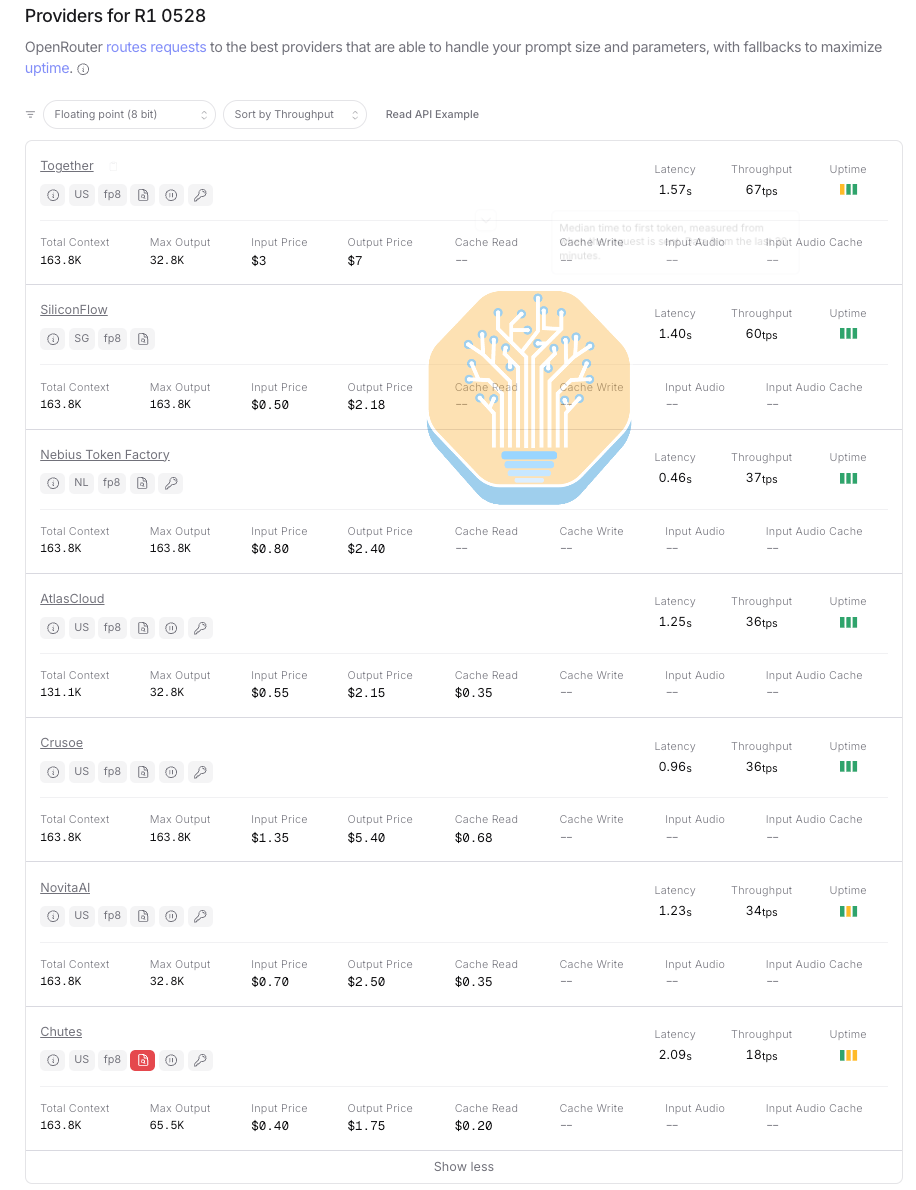
Below is a list on OpenRouter of all inference providers that serve DeepSeek R1 0528 FP8 along with their cost per million input/output tokens and average interactivity listed on. Disregarding Chutes, the middle of the pack provider serves at an interactivity of around 35 tok/s/user.
We can then use real InferenceX data to interpolate the cost per million input/output tokens at an interactivity level of 35 tok/sec/user, which is a reasonable interactivity level given the data above.
As we mention later in the article, this is best understood as baseline data and not completely representative of real-world inference, mainly because InferenceX benchmarks on random data and disables prefix caching. In other words, performance/cost will be at least this good. It is also important to note that there are not data points for each GPU at each interactivity level. Thus we cannot make exact comparisons at each degree of interactivity. We nevertheless think the bar chart comparisons presented below are (very) reasonable interpolations in lieu of using exact data points.
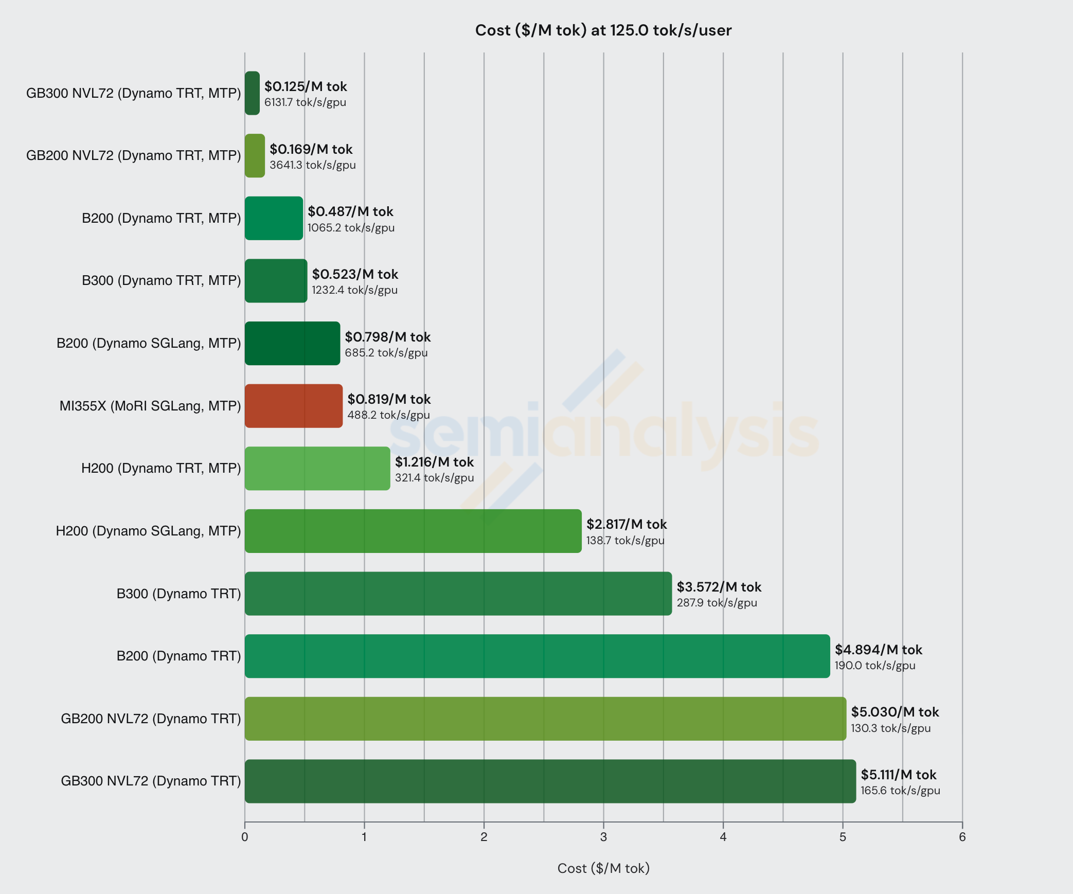
Comparing disagg+wideEP configs at this interactivity level, we see just how effective distributed inference techniques are when it comes to both perf/TCO and overall throughput. We also see how large scale up domains (like GB300 and GB200 NVL72) absolutely dominate in total throughput per GPU.
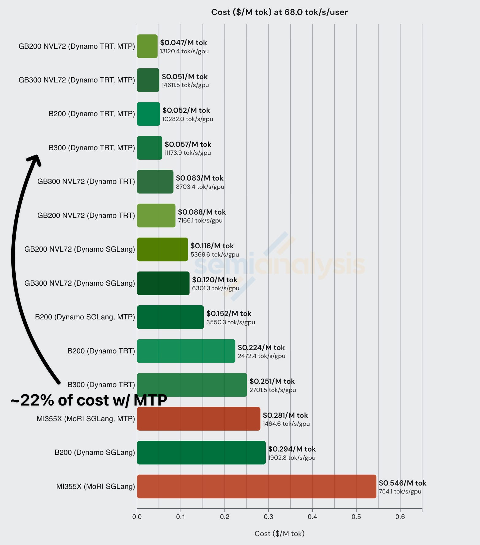
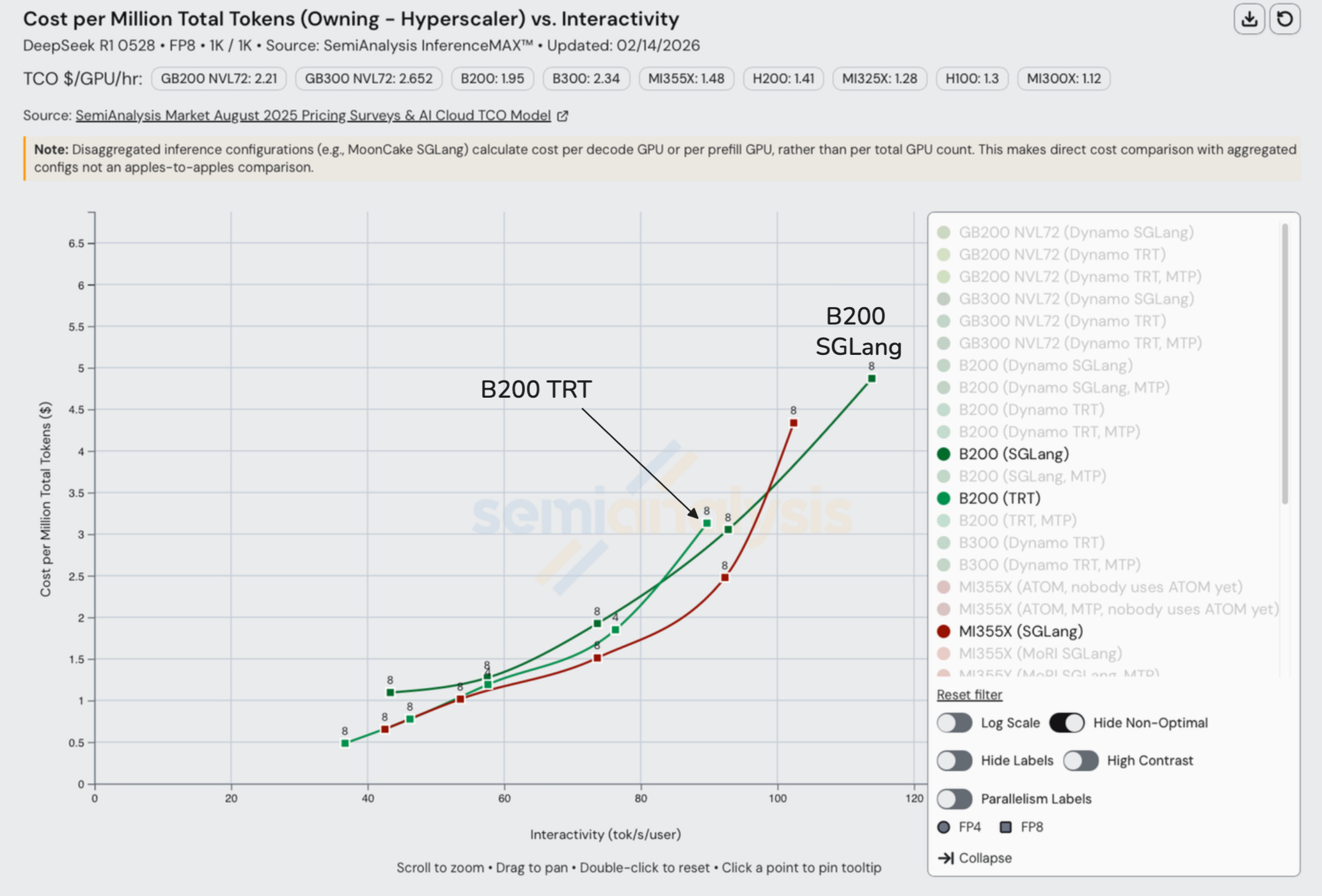
It is interesting to note that at this interactivity level (on an 8k1k workload type), the B200 can achieve the best perf/TCO when MTP is enabled. Below we also list the Total Cost of Ownership (TCO) (Owning – Hyperscaler) for each GPU:


Let’s use the findings above to dig deeper into the unit economics of serving LLMs at scale. From the OpenRouter data above, we see that Crusoe serves at 36 tok/sec/user at $1.35/M input tokens and $5.40/M output tokens. If we assume no cache hits and that Crusoe is using at least H200s with SOTA inference techniques like MTP, disagg, and wide EP, the data above suggests they incur a cost of no more than $0.226$/M input tokens and $2.955/M output tokens for a profit margin of up to 83% gross margin (depreciation counted in cost of goods sold) on input tokens and 45% gross margin on output tokens.
Of course, these assumptions may not be exactly correct and these calculations don’t account for downtime or underutilization, but this gives an idea of some cool math you can do with InferenceX data. More analysis on the economics of inference can be found in the SemiAnalysis Tokenomics Model.
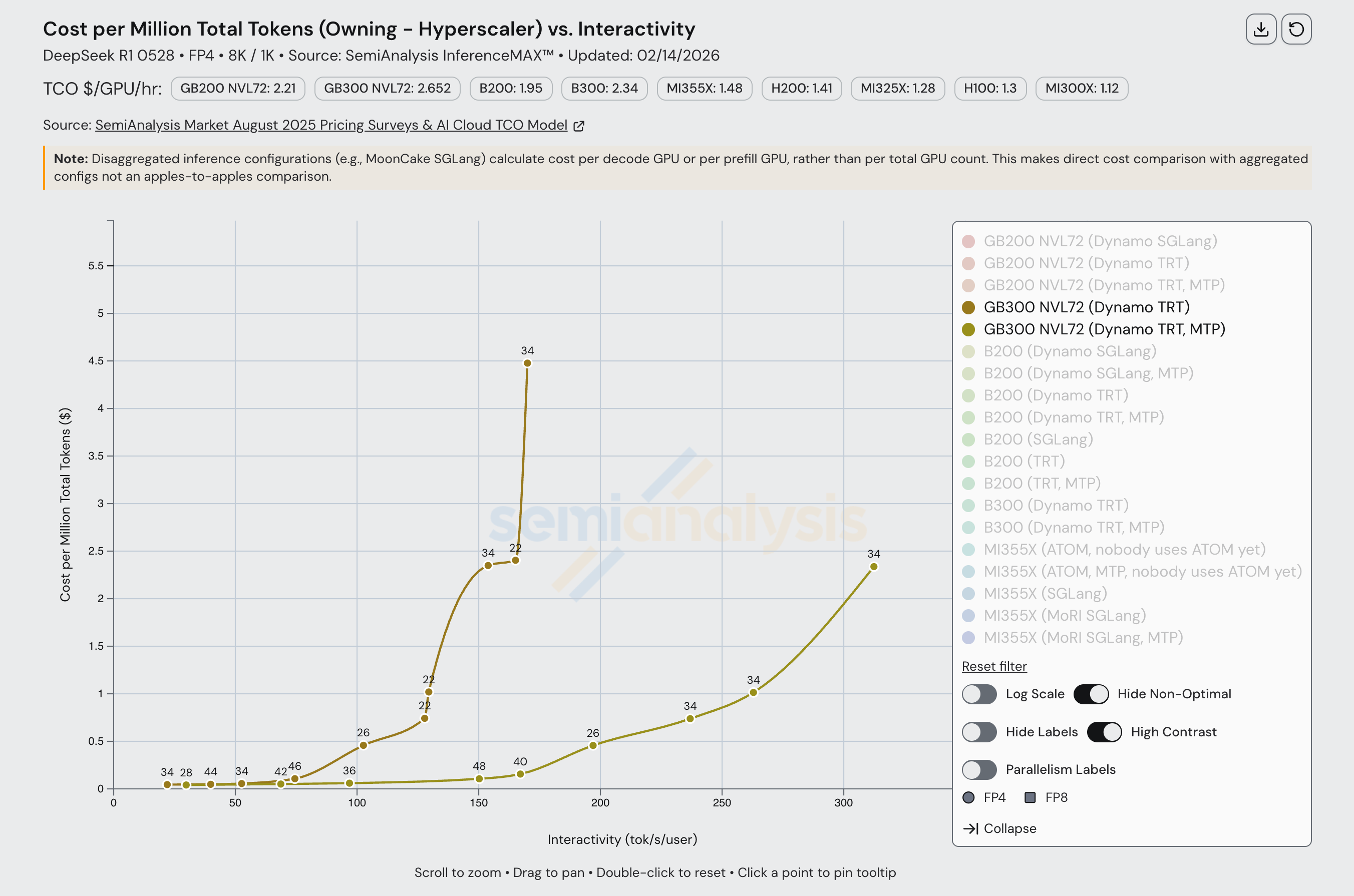
The OpenRouter data also shows Nebius AI Studio (Fast) serving DeepSeek FP4 at 167 tok/sec/user at $2/M input, $6/M output tokens. Adjusting the interactivity level in InferenceX accordingly and we see the following data.


At this high of interactivity, it becomes necessary to employ speculative decoding techniques like MTP to achieve high enough throughput to make inference economical. Luckily, MTP can increase throughput with relatively low risk to overall model accuracy. We will go on to talk more about MTP, and how it can be applied to increase throughput / decrease cost, in later sections of this article.
Lastly, we show one more chart of an FP8 DeepSeek workload served at 125 tok/s/user. This is another low latency workload where MTP considerably improves economic viability. As with the previous example, we note that at these higher ranges of interactivity, the cheapest configs all use MTP.
Nvidia Disagg Prefill and WideEP
EP requires all-to-all communication, where every GPU needs to send tokens to every other GPU. This is extremely bandwidth hungry. Recall that Nvidia’s servers have two separate networking domains – the scale-up NVLink domain, and the Scale-out Domain, usually using InfiniBand or Ethernet as the networking protocol.
NVLink domain (within the NVL72 rack): 72 GPUs connected via NVLink with 900 GB/s uni-directional bandwidth per GPU. This is roughly 7-10x the bandwidth of the InfiniBand/Ethernet based scale-out network.
InfiniBand/RoCEv2 Ethernet (outside of the NVL72 rack): Typically 400-800 Gbit/s per GPU uni-directional (50-100 GB/s). Note that all our testing for Nvidia was conducted on InfiniBand based clusters.
TP shards every layer’s weight matrices across GPUs. This means that every single token at every single layer requires up to two all-reduce communications (one after the column-parallel GEMM, one after the row-parallel GEMM). For EP, all-to-all is done only at MoE layers. Each GPU sends only the tokens routed to each expert. This means cheaper comms across all layers for EP vs TP.
Because EP’s all-to-all communication bandwidth requirements scale with the number of participants, staying within the high-bandwidth NVLink domain before having to cross the slower IB/Eth fabric is better. With NVL72, EP across 72 GPUs is possible without ever leaving NVLink, whereas previous generations (with only 8-GPU NVLink domains) could only do EP across 8 GPUs at NVLink speed before hitting the slower IB/Eth networks.
Wide EP also has a major advantage in weight loading efficiency. For a model like DeepSeek R1, decode is memory-bandwidth-bound: the bottleneck is how fast GPUs can load weights from HBM. With wide EP (e.g., DEP32), 32 GPUs collectively hold and load the 670B weights once, each loading only its shard (~21B). The total HBM bandwidth of all 32 chips is applied to loading a single copy of the model. By contrast, with narrower EP and more DP replicas (e.g., 5xDEP8), each of the 5 replicas needs its own full copy of the 670B weights, that’s 5×670B = 3.35T of redundant weight loading across the system. EP amortizes weights across chips; DP replicates them. This is why wider EP, enabled by high-bandwidth interconnects like NVLink, delivers significantly better throughput per GPU.
Generally, TP is preferred at lower concurrencies due to load balancing. At small batch sizes, EP suffers from uneven token-to-expert routing, leaving some GPUs underutilized while others are overloaded. TP avoids this since each GPU holds a slice of every expert and always gets an equal share of work. At lower concurrency, the cost of this load imbalance outweighs TP’s additional communication overhead.
At higher concurrencies, this tradeoff changes. Expert activation becomes more evenly distributed across larger batch sizes, and EP’s communication and weight-loading advantages dominate over TP’s expensive per-layer all-reduce. In the middle of the curve, hybrid TP+EP configurations balance both concerns using small TP groups within each expert for load balancing while EP is used across the wider set of GPUs to amortize weights and reduce communication.
For higher interactivity levels (low batch size), large scale-up world sizes tend not to deliver stronger performance. B300 disagg over IB has the same performance as GB300 with NVL72, since the workload is latency-bound, not bandwidth-bound. The massive NVLink bandwidth advantage of NVL72 doesn’t matter because not even the much slower IB link is saturated by the tiny batches of tokens in flight.
Prefill/decode disaggregation also plays a role. Prefill is compute-heavy and bursty; decode is memory-bandwidth-bound and steady-state. When they share the same GPUs, they interfere with each other, causing latency jitter and wasted capacity. Separating them onto dedicated GPU pools lets each run a workload matched to its characteristics, improving effective utilization. This is why disaggregated B200 configs outperform single-node B200 in the middle of the throughput-interactivity curve. PD separation combined with wider EP across more GPUs over IB amortizes weights more efficiently than cramming both phases onto a single 8-GPU node.
Jensen Under Promising and Overdelivering - Hopper vs Blackwell vs Rack Scale NVL72
At GTC 2024, Jensen was on stage promising up to 30x performance gains from H100 to GB200 NVL72, everyone thought it was classic marketing lookmaxxing and would not be achievable in real world. Many looked to come up with labels for this perceived use of a reality distortion field so they could crack more Jensen Math jokes. Indeed – we did point to the comparison of 30x performance difference between the worst case for H200 on FP8 to a reasonable case of the GB200 on FP4.

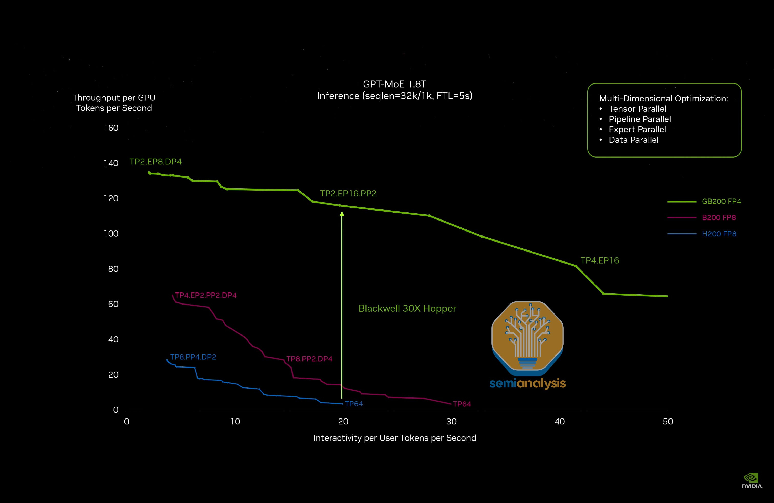
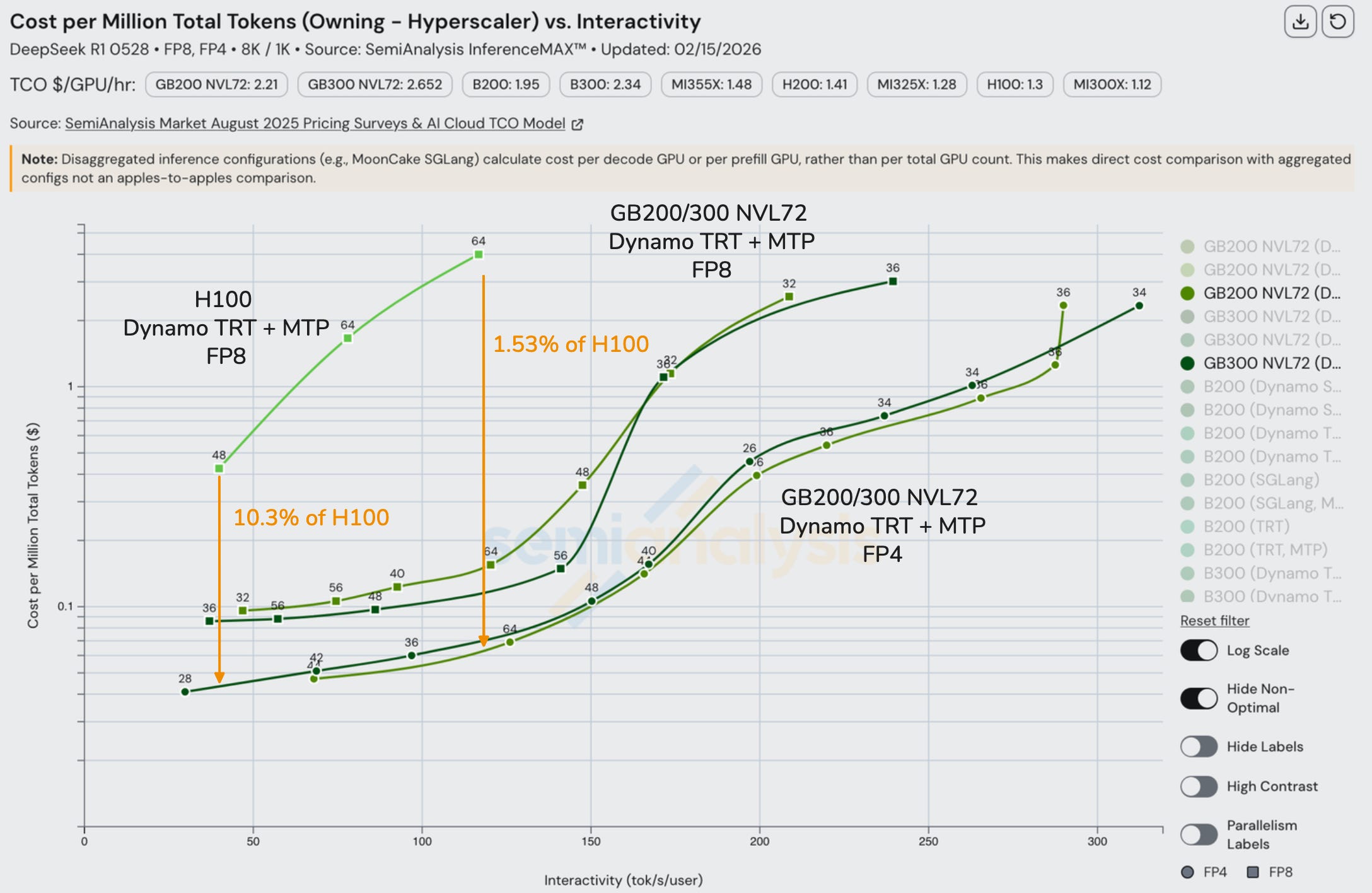
But it turns out the joke is on them. Fast forward almost two years later, and we can now see that it wasn’t marketing hype lookmaxing after all, and Jensen was actually under promising on Blackwell performance the whole time. From our testing, Blackwell is so good at large scale MoE inferencing compared to even a strong H100 disagg+wideEP FP8 baseline that it, at 116 toks/s/user, delivers up to 98x better perf on GB200 NVL72 FP4 and up to 100x better perf on GB300 NVL72 FP4! Maybe the new Jensen Math rule is that he delivers double whatever he promises in terms of token throughput. The more you spend, the more you save indeed!
Even when factoring in the increased total cost of ownership of Blackwell and Blackwell Ultra, we see a 9.7x(40 tok/s/user) up to 65x(116 tok/s/user) improvement in tokens per dollar compared to Hopper. You can explore Hopper vs Blackwell performance in detail on our free website. Blackwell performance is so good compared to Hopper that we needed to an log scale to our dashboard in order to visualize it.
As mentioned earlier in the article, B300 servers only connect at most 8 GPUs using the 900GByte/s/GPU NVLink scale-up network whereas GB300 NVL72 servers connect 72 GPUs using the NVlink scale-up network. So when we need more than 8 GPUs (but less than 72 GPUs) for the inference setup, we need to bring in multiple nodes of B300 servers to form our inference system which means communications falls back to the lower InfiniBand XDR scale-out network featuring 800Gbit/s (uni-di) per GPU of bandwidth. Compare this to a rack scale GB300 NVL72 which connects 72 GPUs over NVLink delivering 900GByte/s (uni-di) per GPU of bandwidth and we can see that the rack-scale server allows the GPUs in the inference setup to talk to each other with over 9x higher bandwidth compared to the case of the multiple nodes of B300 servers.
Admittedly the GB300 NVL72 has a higher all-in cost per GPU, but this only reduces the bandwidth per TCO advantage to being 8x faster. The bandwidth advantage of the rack-scale architecture directly drives a much lower cost per token. Google TPU, AWS Trainium and Nvidia are the only AI chips to have rack scale system designs deployed today. Engineering samples and low volume production of AMD’s first rack scale MI455X UALoE72 system will be in H2 2026 while due to manufacturing delays, the mass production ramp and first production tokens will only be generated on an MI455X UALoE72 by Q2 2027.
Blackwell vs Blackwell Ultra
On paper, the newly released Blackwell Ultra has the same memory bandwidth as Blackwell, the same FP8 performance and only 1.5x higher FP4 performance, but when measuring we actually see up to 1.5x better FP8 performance on the Blackwell Ultra, though we only see 1.1x better performance on FP4. This may be due to Blackwell Ultra being a newly released GPU, meaning software is not fully optimized yet.


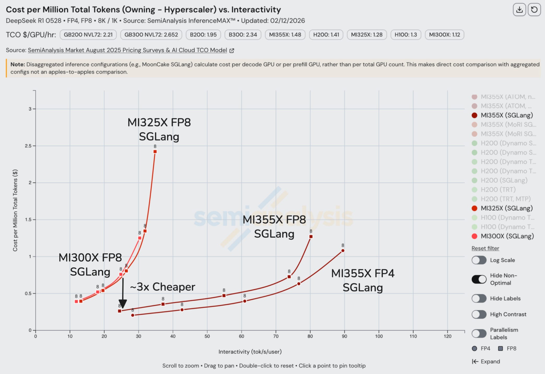
MI355X vs MI325X vs MI300X
On AMD SKUs, we see up to 10x better performance on the MI355X vs the MI300X. AMD has only gotten DeepSeek SGLang Disaggregated Inferencing to work on the MI355X so far AMD has not submitted MI300X or MI325X disaggregated inferencing results, potentially due to software issues on older SKUs that are still being solved.
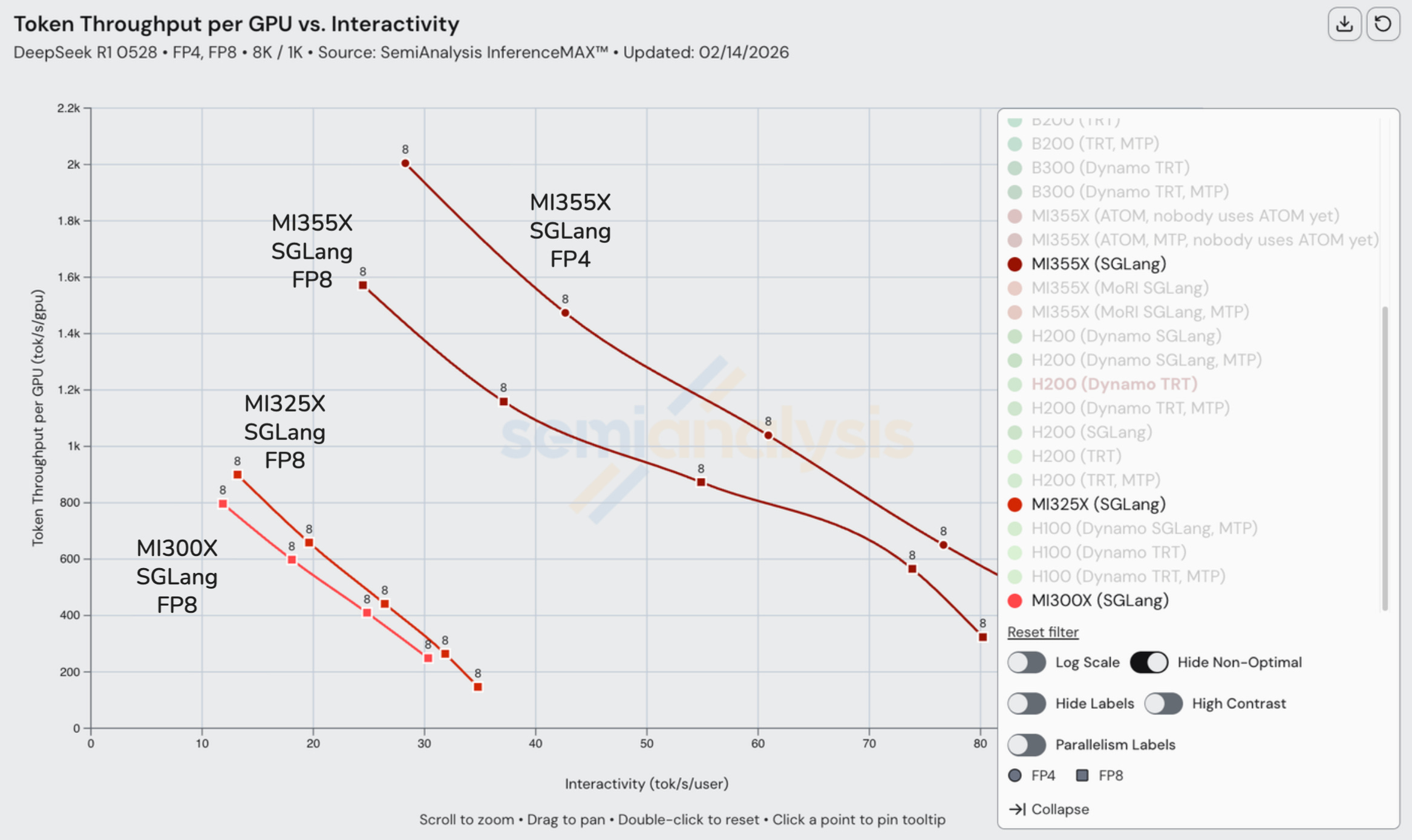

Turning to cost, for DeepSeekR1 on FP8, at an interactivity of 24 tok/s/user, the MI355X delivers inferences a cost that is slightly less than 3x cheaper than for the MI325X. The throughput of each GPU is slightly less than 4 times that of MI325X.
AMD Composability Issue on FP4, Distributed Inferencing and Wide Expert Parallelism
While AMD performs somewhat decently on single node FP4 and performs competitively to B200 SGLang on FP8 distributed inferencing, the issue with the current AMD open source inferencing stack is that, while individual inference optimizations perform well, real customers deploy with multiple optimizations composed together. Top tier AI labs are all using FP4 with disaggregated inferencing with wide expert parallelism all enabled at the same time, and this is where the issue occurs.
AMD software is still not meeting the mark, and the theoretical speed of light modelling at SemiAnalysis and at AMD show that for FP4, disaggregated inferencing with wide expert parallelism should perform better than inference on a single node of MI355X. Unfortunately, Software continues to be a massive bottleneck for AMD GPUs. AMD management needs to continue to sharpen resource allocation of their engineering talent, for instance, re-allocate their engineering resources away from pet single node projects that nobody uses like ATOM towards fixing the aforementioned issues with composability of inference optimizations between disaggregated inferencing, wide expert parallelism and FP4. The current subpar software is due to lack of focus and incorrect prioritization of where the industry already is at. All top tier labs are already using disaggregated inferencing and wide expert parallelism; AMD needs to stop focusing on single node and heavily invest focus into multi node inferencing for open source solutions.
AMD is more than six months behind on open source distributed inferencing and wide expert parallelism and FP4 composability as shown by Nvidia and SGLang team showing off their NVFP4 performance on DeepSeek six months ago.
AMD ATOM Engine
AMD has launched a new inference engine called ATOM. Atom can deliver slightly better single node performance, but it is completely lacking on a lot of features that makes it unusable for real workloads. One such example is that it does not support NVMe or CPU KVCache offloading, tool parsing, wide expert parallelism, or disaggregated serving. This has led to zero customers using it in production. Unlike Nvidia’s TRTLLM which generates billions of tokens per hour globally at companies like TogetherAI, etc and does support tool parsing and other features, there are no token factories currently using ATOM due to the lack of the aforementioned features.
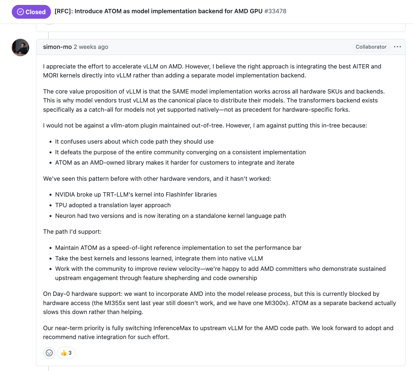
Furthermore, maintainers of open-source inference engines like vLLM are disappointed in AMD due to a lack of engineering and GPU resources provided by AMD. For example, Simon Mo, lead vLLM maintainer, states in this GitHub RFC that there is still no working MI355X that he can add to vLLM CI, hence the poor user experience. There are currently zero Mi355X tests on vLLM, while NVIDIA’s B200 has many tests on vLLM. Similarly, there are still not enough MI300X CI machines on vLLM. Upstream vLLM needs at least 20 more MI300 machines, 20 more MI325 machines and 20 more MI355X machines to reach the same level of usability as CUDA.
We at SemiAnalysis have been trying to get AMD to contribute more compute to vLLM and have had some success on that within the couple weeks. vLLM will start to get a couple of MI355X machines such that they can bring their CI test parity from 0% to non-0%. We will talk more about AMD’s previous lackluster contribution towards vLLM, SGLang, PyTorch CI machine situation & how Anush started to fix it in our upcoming State of AMD article. At SemiAnalysis, we will have internal dashboard to track the # of tests & quality of tests that AMD & NVIDIA runs on vLLM, SGLang, PyTorch, & JAX.
Moreover, the vLLM maintainers say that they cannot support day 0 vLLM support for ROCm due to this issue of lack of machine resources. This huge disparity in time to market continues to lead to ROCm lagging behind and leaving a huge opening for Nvidia to continue to charge an insane 75% gross margin (4x markup on cost of goods).
Lastly, AMD has not had enough committers “who demonstrated sustained upstream engagement through feature shepherding and code ownership” and has a lack of reviewers that can review their own code. This is why the pace of development on ROCm vLLM has been much slower than for CUDA vLLM.
There are many talented 10x engineers at AMD that work on ATOM and we would encourage AMD management to think about re-deploying these 10x engineers towards working on libraries and frameworks that people actually use, such as vLLM and SGLang.
As we mentioned earlier, AMD also needs to prioritize addressing composability issues with FP4, wideEP and disaggregated serving as opposed to overly focusing on optimizing FP4 for a single node.
Multi Token Prediction (MTP)
Speculative decoding reduces the cost of autoregressive generation by using a small, inexpensive draft model to propose several tokens ahead. The large model then checks the proposed tokens in a single forward pass that resembles a prefill computation. For a given input sequence length, a single forward pass can take roughly the same time when the input has N more tokens. Speculative decoding uses this property to run inference on a smaller model to draft multiple tokens for the main model to verify with a single forward pass, producing at most N additional tokens in a similar time budget.
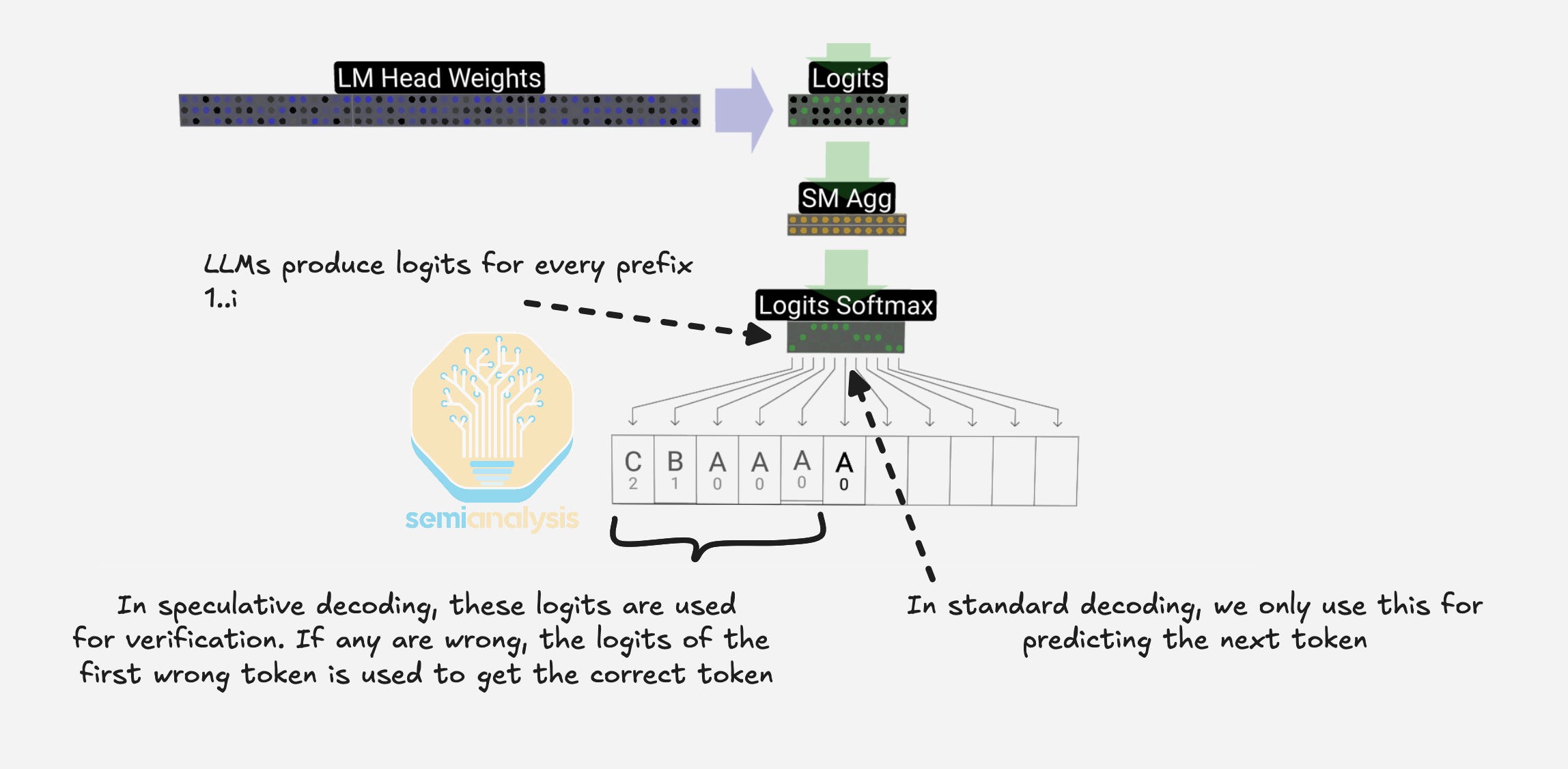
This assumption regarding additional token production with the same time budget is strongest for dense models because batched verification can reuse the same weight stream across multiple positions. For Mixture-of-Experts models, different tokens may route to different experts, so verifying multiple draft tokens can activate more experts than single-token decoding and force additional expert weights to be fetched from memory. As shown in the Mixtral 8x7B Instruct model results in the EAGLE paper, this extra memory traffic erodes bandwidth savings and can make verification notably comparable to a standard decoding step.
Multi-token prediction pursues similar benefits without requiring a separate draft model. Auxiliary prediction heads are added to the model architecture, so a single model can propose several future tokens from the same underlying representation. This improves distribution alignment because the proposals come from the same model that ultimately scores them. Multi-token prediction also avoids the operational complexity of serving an additional model while still enabling multi-token generation strategies but requires the MTP heads to be pretrained alongside the main model.
Across all SKUs, enabling MTP results in performance gains. By making use of the typically unused logits to verify the extra tokens, minimal compute overhead is added, saving extra expensive weight loads during decode.
At large batch sizes, the inference regime is less memory-bandwidth bound compared to for low batch sizes. Since speculative decoding (including MTP) works by trading excess compute for fewer memory-bound decoding steps, this extra verification work from speculative tokens may not fit cleanly into slack, resulting in smaller improvements at high batch sizes.
In terms of cost, MTP can drive huge cost savings, in the below table, we see that DeepSeek-R1-0528 run on FP4 using Dynamo TRT costs $0.251 per million total tokens, but enabling MTP can push costs down dramatically to only $0.057 per million total tokens.
In all configs, when all else is held equal, using MTP with DeepSeek R1 increases interactivity with no significant impact on model accuracy. This is in line with the DeepSeek V3 tech report findings.
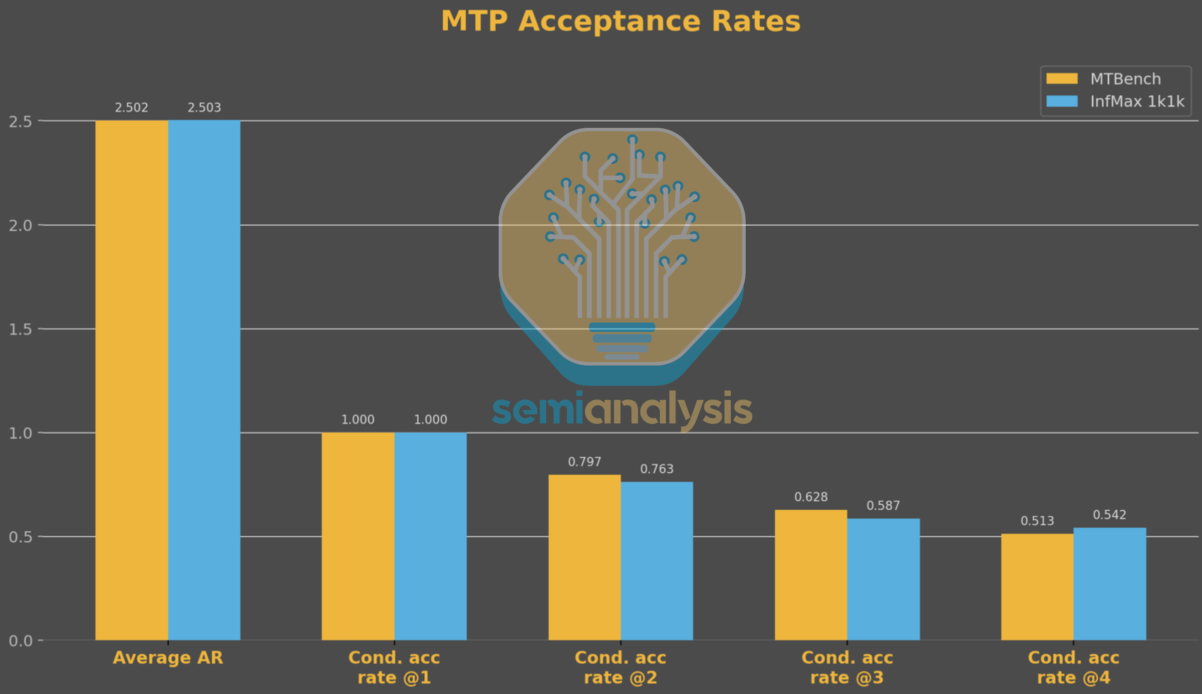
Regarding the validity of MTP performance numbers, one may argue that the distribution of a synthetic dataset may not resemble real data. However, comparing MTP acceptance behavior between MTBench and our 1k1k benchmark, we see a very similar distribution confirming that our InferenceX benchmark is a good proxy for real world production performance. That said, InferenceX is not perfect and we are always looking to improve. If you want to be part of the mission, apply to join our special projects team here.
Accuracy Evaluations
Throughput optimizations can sometimes quietly trade off accuracy (e.g. via aggressively relaxed acceptance rates, decoding tweaks, numerically unstable kernels, or endpoint misconfiguration). Without evals, a misconfigured server (truncation, bad decoding, wrong endpoint params) can still produce great throughput numbers but deliver garbage answers. For example, this additional layer of checks has helped us discover issues with some DP attention implementation for GPT-OSS.
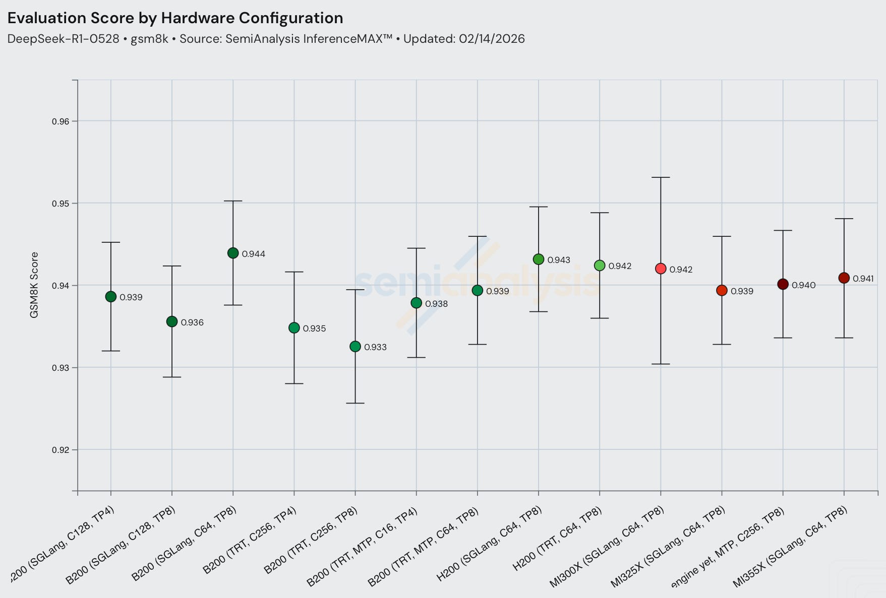
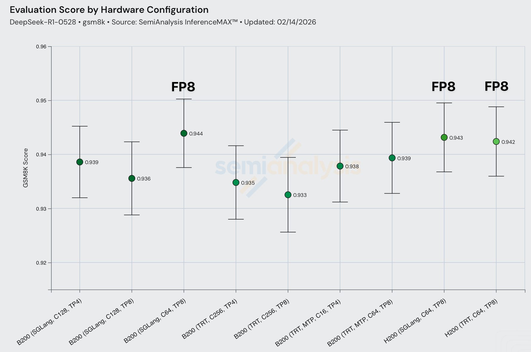
Each representative throughput config now has an associated numerical accuracy check. Currently we are only using GSM8k, but being a very easy benchmark, the evaluation scores may not change much from differences in numerical calculation, and a harder benchmark may have a larger delta with respect to numerical accuracy. Thus, we plan to expand towards harder ones in the future, such as GPQA, HLE, MATH-500, SWE-Bench verified.
Another form of performance-accuracy tradeoff is quantization. Serving models at lower precision may result in worse model outputs. For DeepSeek R1, FP8 runs have very slightly higher evaluation scores than FP4. Note that GSM8k evals are saturated and often during QAT/PAT it is calibrated to common popular GSM8k, MATH-500, etc, leading to sometimes evals showing great results while real world end user evaluation being subpar. If we want to be part of the team to figure out how to properly evaluate inference engine accuracy, apply to join the mission here.
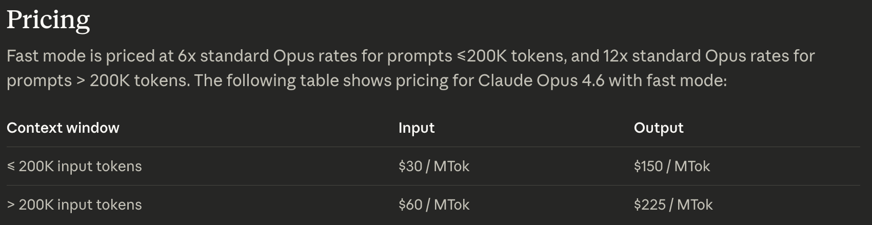
Anthropic Fast Mode Inferencing Explained
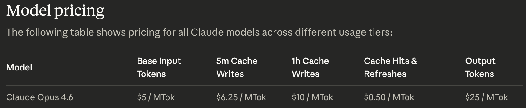
Anthropic recently released “fast mode” alongside Opus 4.6. The value proposition: the same model quality at roughly 2.5× the speed, for around 6–12× the price. Both figures might seem surprising, and some users have speculated that this must require new hardware. It doesn’t. In fact, this is just the fundamental tradeoff at play. Any model can be served at a wide range of interactivity levels (tokens/sec per user), and the cost per million tokens (CPMT) shifts accordingly. Mercedes makes metro busses as well as race cars, to follow long with our analogy.
Bean counters may think that fast mode is more expensive, but when looking at it through a total cost of ownership lens, fast mode is actually way cheaper for some situations. For example, a GB200 NVL72 rack can cost 3.3 million dollars, and as such, if claude code agentic loops (which runs on Trainium in production) that tool use call NVL72 racks, and these racks run inference 2.5x slower, you would need 2.5x more racks to deliver inference, meaning that not enabling fast mode would cost close to 5 million dollars in extra spend.
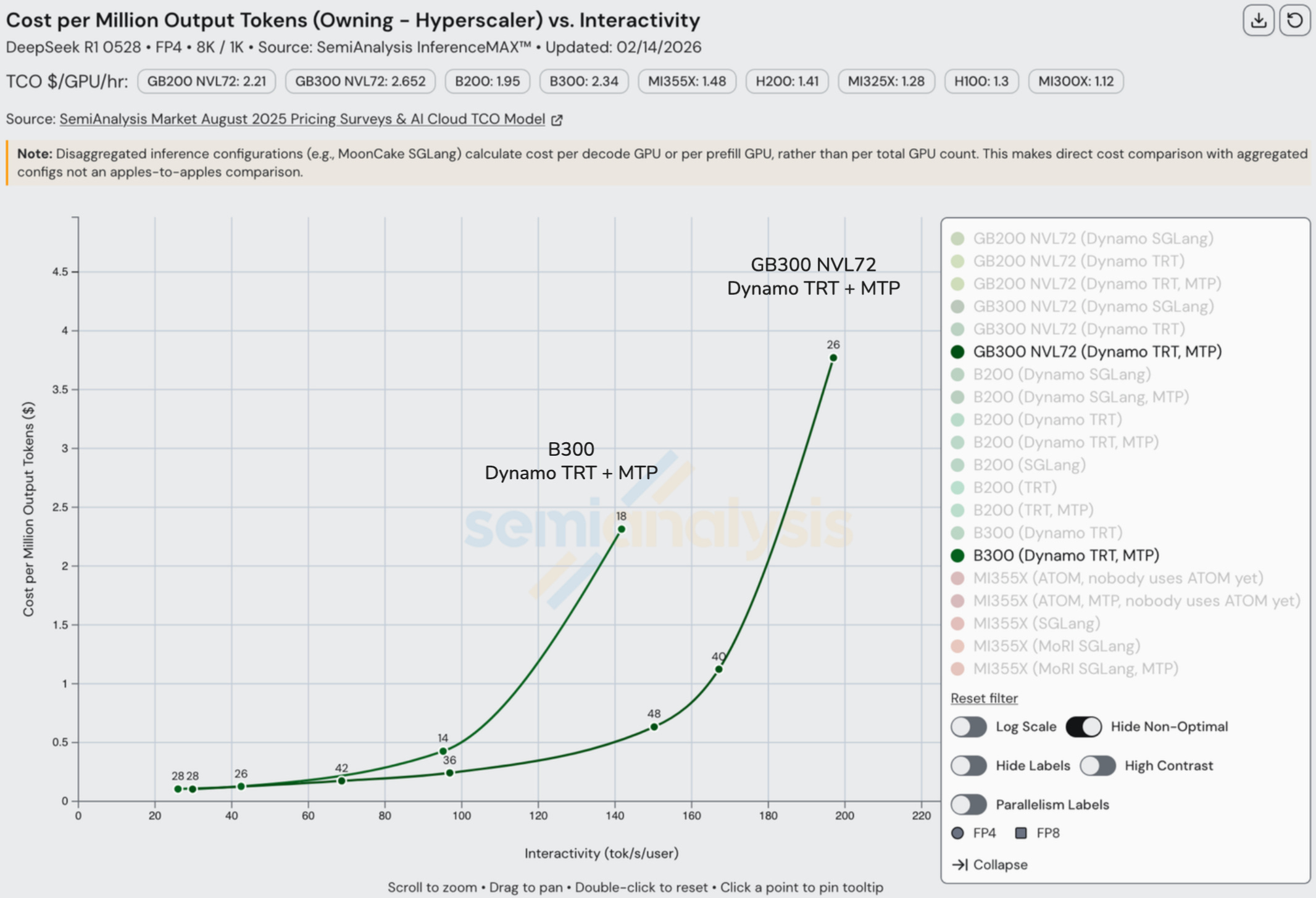
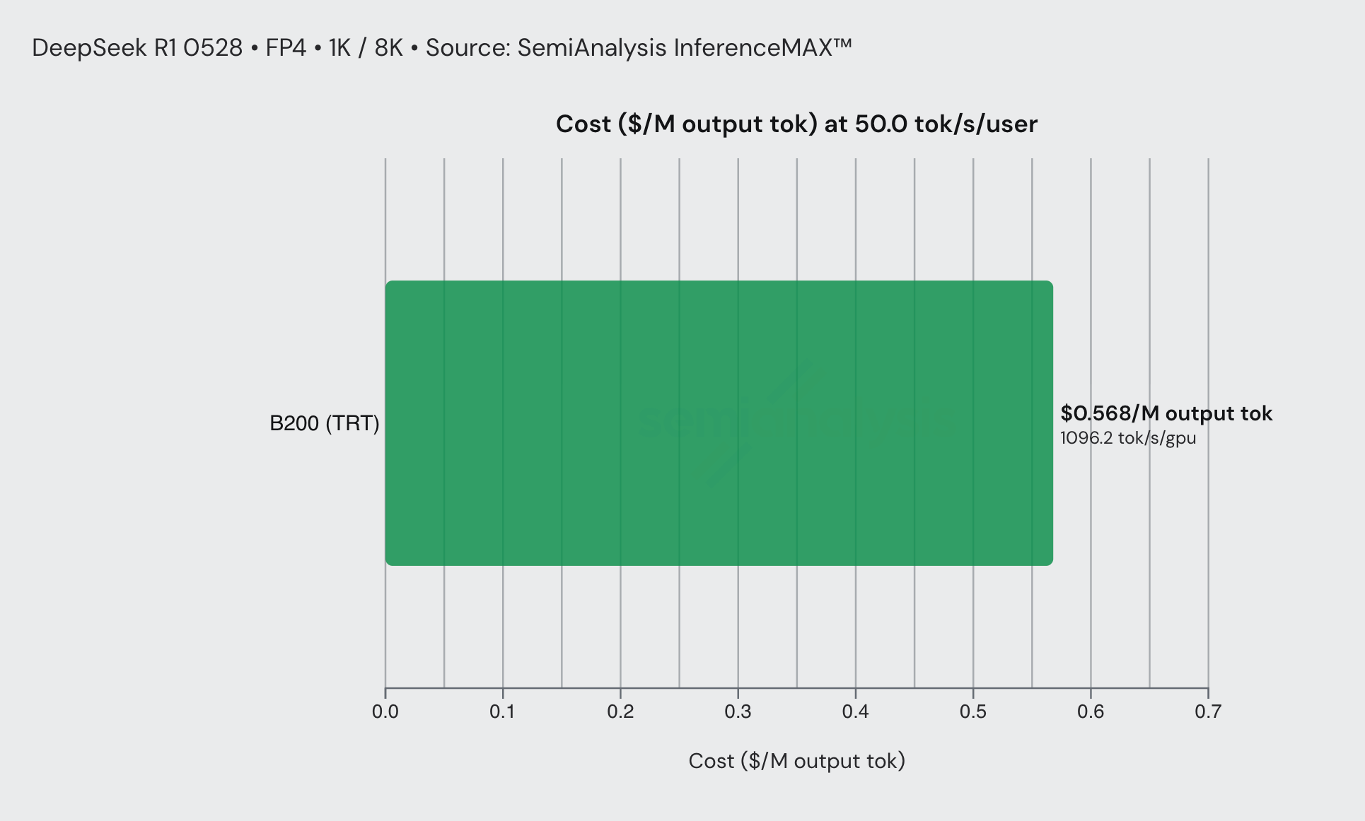
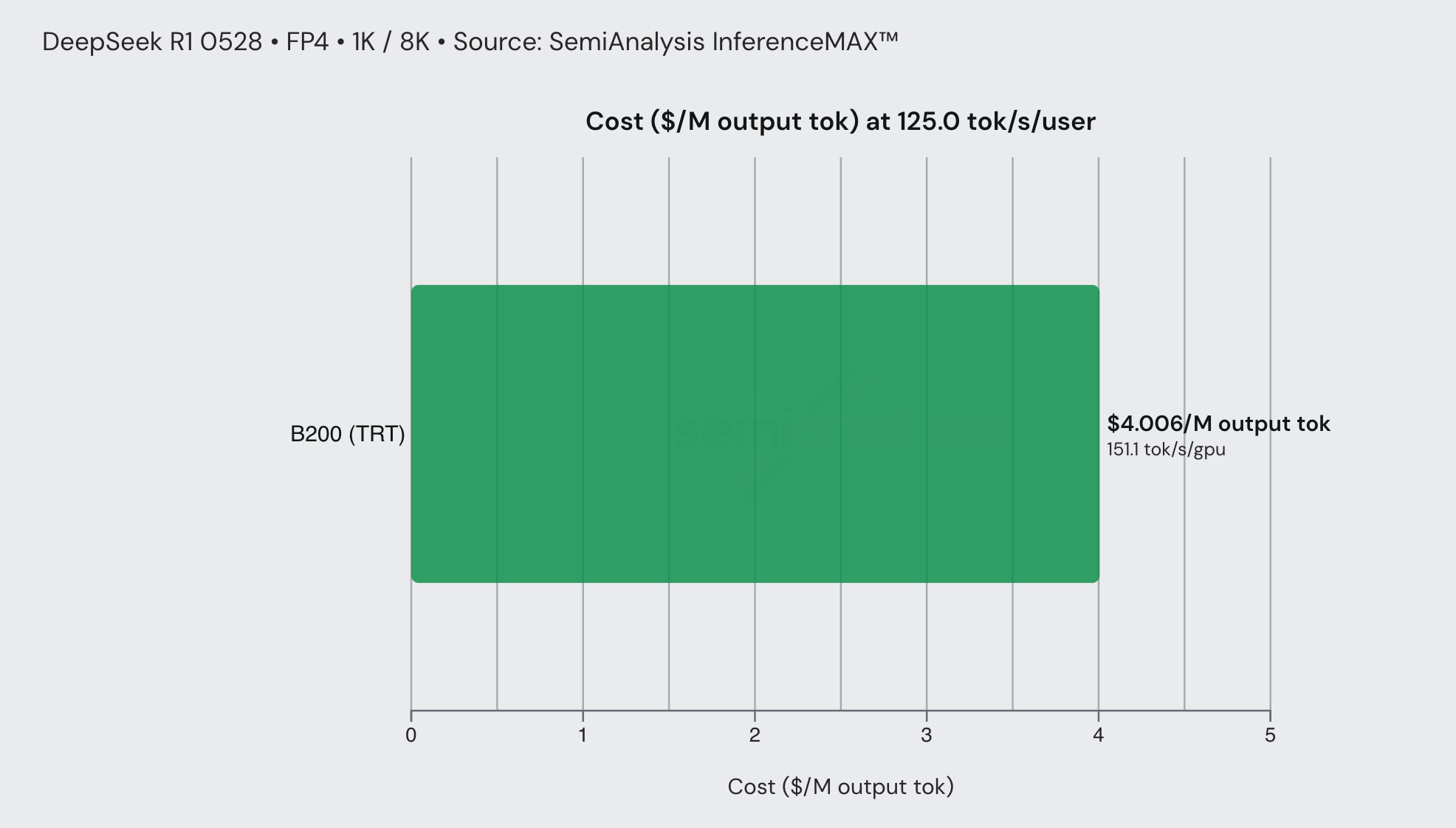
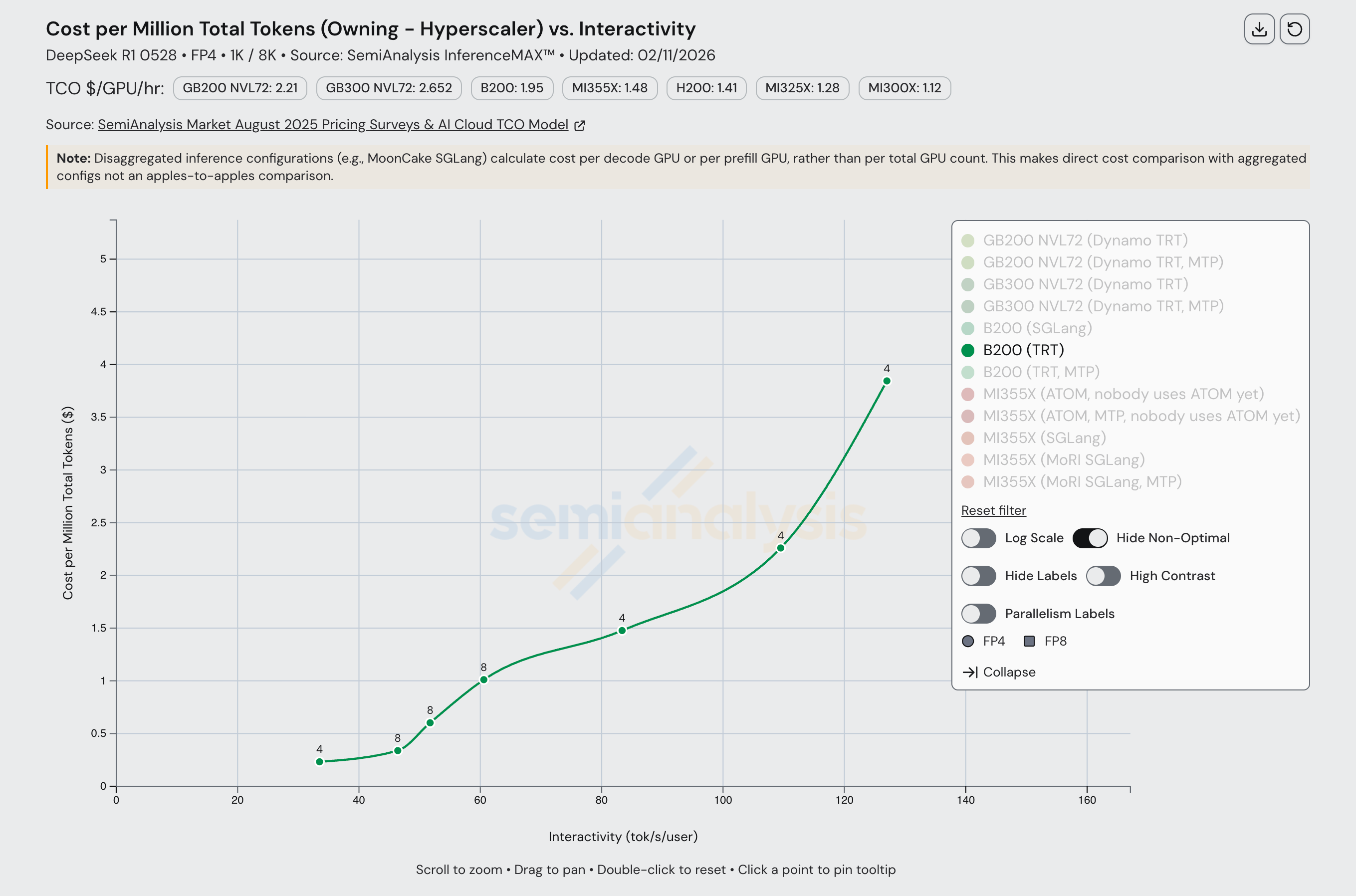
Consider a DeepSeek R1 0528 FP4 coding workflow served on B200s with TRT-LLM. At an interactivity of 50 tok/sec/user, inference cost is approximately $0.56/M output tokens. At an interactivity of 125 tok/sec/user, this rises to around $4/M output tokens, a 2.5× speed increase for a ~7× price increase, closely mirroring what we see with Anthropic’s fast mode. Note that this assumes DeepSeek R1 is similar to Opus 4.6, which isn’t the case. Still, the general principle holds true.
This follows directly from the fundamental latency-throughput tradeoff in LLM inference. At high batch sizes, GPUs achieve better utilization and greater total token throughput, meaning more users served concurrently and lower cost per token. At low batch sizes with greater parallelism per request, each user gets faster responses, but total token throughput drops. Since the hourly cost of the accelerators is fixed regardless of how they’re used, lower throughput means fewer tokens over which to amortize that cost, and thus a higher price per token.
In short, fast mode isn’t necessarily a hardware story, but merely the natural consequence of trading throughput for latency on the same GPUs.
Furthermore, we observe that inference optimization techniques such as speculative decoding, as explained earlier, can directly lead to cheaper inference; no new chips are required.
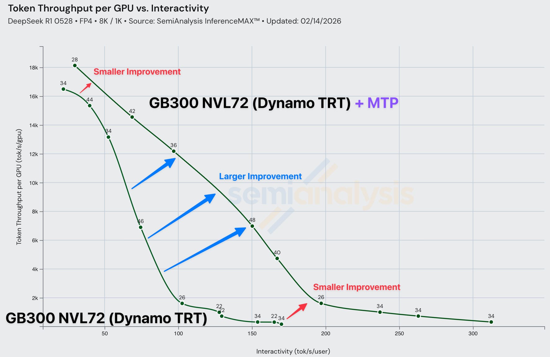
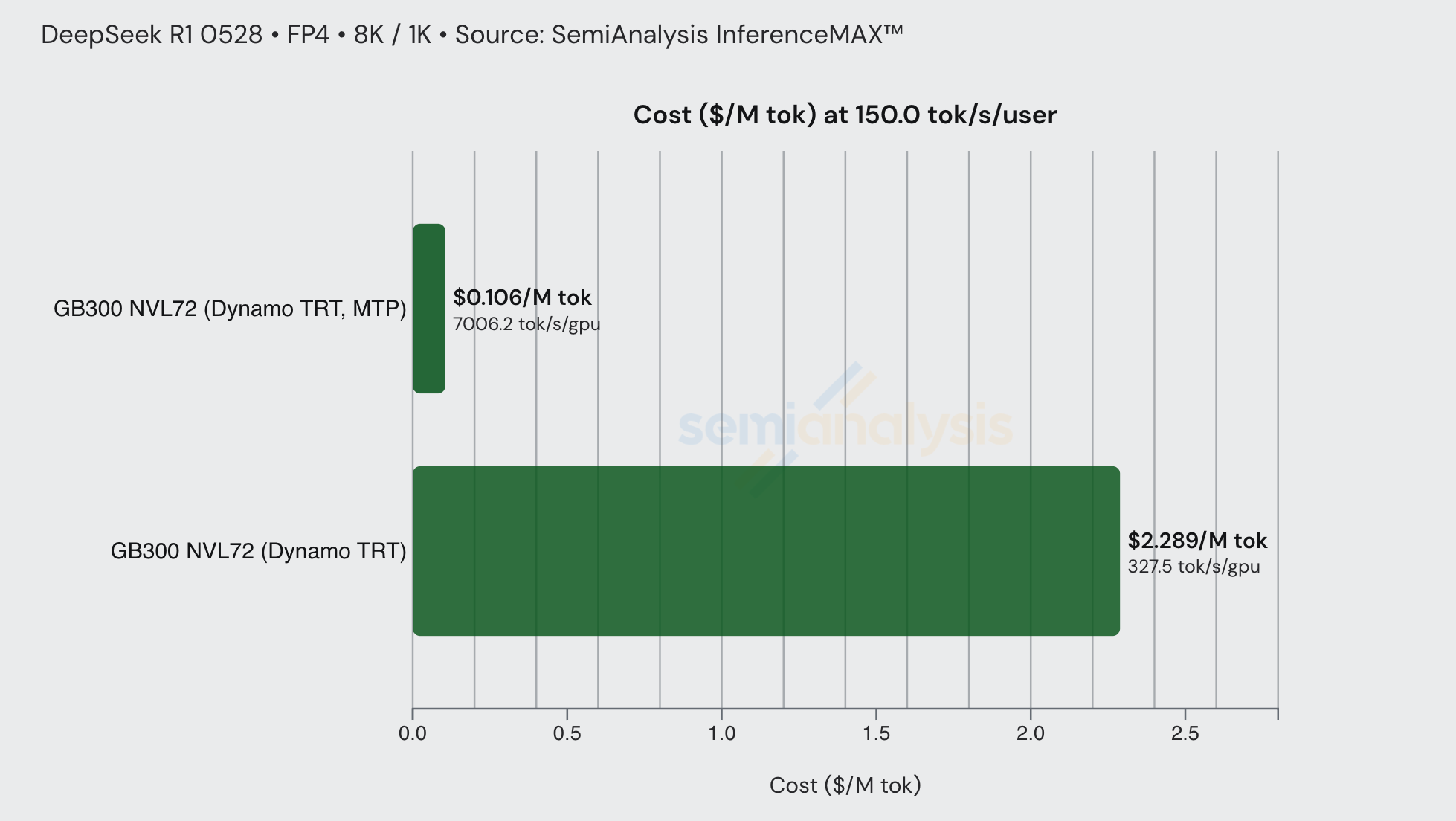
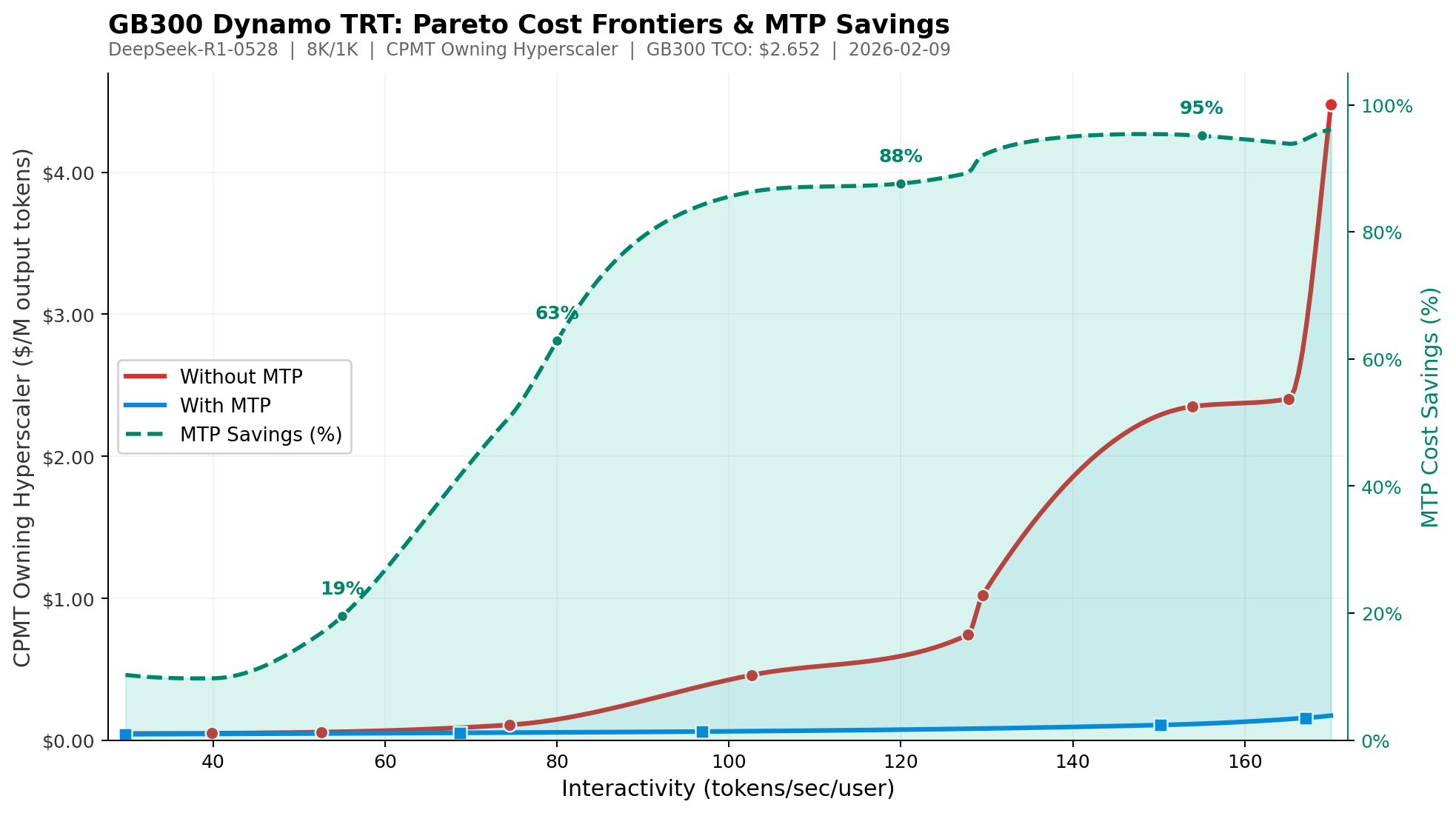
Take the following example, DeepSeek R1 FP4 on an 8k/1k workload. At an interactivity level of 150 tok/sec/user, the baseline GB300 Dynamo TRT cost per million tokens is approximately $2.35, whereas enabling MTP decreases the price to approximately $0.11. This is a ~21x price decrease at this interactivity level simply by employing an inference optimization technique.
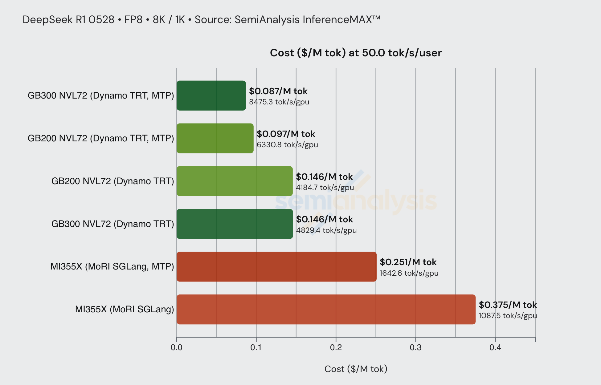
Fixing an interactivity level of 50 tok/sec/user, we further see how much MTP can effectively decrease CPMT across a variety of chips.
Wide Expert Parallelism (WideEP) and Disaggregated Prefill
In this section, we will go deeper on expert parallelism and go on to explain what wide expert parallelism is. We will then explain the idea of Disaggregated Prefill, how it is different from WideEP, and how WideEP and Disaggregated Prefill are used in unison to achieve SOTA performance.
WideEP
By now, most frontier AI labs employ Mixture of Experts (MoE) model architectures as opposed to dense. In MoE architectures, only a subset of “experts” are activated for each token. For instance, DeepSeek R1 has 671B total parameters, but only 37B active parameters. Specifically, DeepSeek R1 has 256 routed experts (and 1 shared expert) with each token being routed to 8 distinct experts. This architecture lends itself naturally to expert parallelism (EP), which evenly distributes expert weights across some number of GPUs.
Consider serving DeepSeek R1 on a single 8-GPU server. At 671B parameters, some form of parallelism is required to fit the model across available HBM. The naive approach is tensor parallelism (TP), which shards every weight matrix across all GPUs. This works well for dense models but ignores the sparse activation pattern of MoE. With TP=8, each expert’s weights are sharded across all 8 GPUs, meaning every expert activation requires an all-reduce across all GPUs & the reduction dims of the GEMM is smaller leading to lower arithmetic intensity, even though only 8 of 256 experts activate per token. TP treats each expert like a dense layer, paying full cross-GPU communication cost while the model’s sparsity goes unexploited.
Expert parallelism takes a more well-suited approach, assigning whole experts to individual GPUs. With EP=8, we divide the 256 experts per layer across 8 GPUs for a total of 32 experts/layer/GPU. Each GPU holds approximately 1/8th of the expert weights plus a full replica of the non-expert weights (attention projections, embeddings, normalization, and the shared expert). Since roughly 90%+ of DeepSeek R1’s parameters are routed expert weights, EP captures most of the memory savings, and replicating the remaining less than 30B non-expert parameters across all 8 GPUs is affordable.
The forward pass proceeds in two phases per layer. During attention, each GPU acts as an independent data-parallel rank, processing its own subset of requests using its replicated non-expert weights, no inter-GPU communication is needed. During the MoE phase, a lightweight router determines which experts each token requires, and tokens are dispatched to the appropriate GPUs via all-to-all communication. Each GPU executes its local experts on only the tokens routed to it, and results are returned via a second all-to-all.
The obvious way to scale is replication: deploy N independent EP8 instances across N nodes. Each instance serves requests independently with no cross-node communication. This scales throughput linearly, but each GPU still holds 32 experts per layer, and each token activates at most 8 of those 32 local experts. 75% of expert weights sit cold in HBM.
Wide expert parallelism (WideEP) takes a different approach by scaling EP across nodes rather than replicating independent instances. On a 64-GPU cluster (8 nodes), DP64/EP64 places only 256/64 = 4 experts per layer per GPU, each still holding a full replica of the non-expert weights. During the MoE phase, tokens from all 64 DP ranks are dispatched via all-to-all to the GPUs hosting their routed experts.
This yields three compounding benefits over the single-node EP8 baseline. First, reducing expert footprint from 32 to 4 experts/GPU frees substantial HBM for KV cache, directly increasing per-GPU batch size capacity. Second, 64 DP ranks funneling tokens through fewer experts per GPU increases tokens-per-expert, raising arithmetic intensity (more FLOPs per byte of weights loaded) and improving compute utilization. The same expert weights service 8x more tokens per step. Third, aggregate HBM bandwidth scales linearly with GPU count; 64 GPUs loading expert weights simultaneously provide 8x the memory bandwidth of a single node, reducing memory bottleneck.
The above configurations use only DP+EP (also known as DEP), where each GPU holds a full replica of all non-expert weights. As GPU count grows, this replication becomes increasingly wasteful. On a 64-GPU DP64/EP64 deployment, every GPU stores an identical copy of the ~40B non-expert parameters.
Adding tensor parallelism within groups of GPUs addresses this. In an EP64/DP8/TP8 configuration, the 64 GPUs are organized into 8 DP groups of 8 GPUs each. Within each TP group, the attention projections, shared expert, normalization, and LM head are sharded 8 ways, so each GPU holds only 1/8th of the non-expert weights. Across the full cluster, the 256 experts are still distributed one-per-4-GPUs as before.
Pure DEP has a single communication pattern: all-to-all for expert routing. Adding TP introduces a second all-reduce within each TP group for the attention and non-expert computations. The key design principle is to place TP groups within a single node, where NVLink or MNNVL provides high-bandwidth interconnect, and run EP/DP across nodes, where the all-to-all communication pattern can tolerate higher latency.
As always, the tradeoff is that of throughput versus latency. TP=8 within a group means those 8 GPUs now share a batch and must synchronize every decode step, reducing effective DP degree from 64 to 8. Per-GPU batching independence on the attention side is lost. But each DP group now processes attention 8x faster per step, since the matmul is split 8 ways across the TP group. Per-token latency drops while peak concurrency also drops, sliding the configuration along the latency-throughput Pareto frontier relative to pure DEP.
Disaggregated Prefill
Disaggregated prefill, sometimes referred to as prefill-decode (PD) disaggregation, is the process of performing prefill and decode phases of LLM inference on separate nodes. Prefill occurs when a request is first processed, and a forward pass is computed on all tokens at once, thereby “prefilling” the KV cache for this request. This is a compute-intensive operation as all tokens feed through the forward pass in parallel. Tokens are then generated or “decoded” one at a time, loading the KV cache from HBM at each decode step. This is a memory-intensive process as the growing KV cache is constantly being loaded.
In traditional single-node inference, engines interleave prefill and decode on the same GPUs. Incoming prefill requests stall in-flight decode batches, increasing both time-to-first-token and inter-token latency. Chunked prefill mitigates this by breaking long prefills into smaller pieces, but the fundamental resource contention remains. Disaggregated prefill eliminates this entirely!
Disaggregation also enables independent scaling and optimization of each phase. With separate nodes, each phase can be tuned independently: different parallelism strategies, different batch sizes, and different memory allocation ratios. The ratio of prefill to decode nodes can also be matched to the workload’s input-output length ratio. For instance, prefill-dominated workloads (long input, short output e.g., summarization, RAG, agentic coding with large context windows) allocate more prefill instances. Decode-dominated workloads (short input, long output e.g., chain-of-thought reasoning, long-form generation) allocate more decode instances. Workloads with high cache hit rates also tend toward more decode, since reused KV cache entries from shared system prompts or multi-turn conversation history skip prefill entirely.
The key cost of disaggregation is KV cache transfer. After prefill completes, the full KV cache for that request must be transmitted from the prefill node to the decode node before the first decode token can be generated. For a model like DeepSeek R1 with 61 layers and FP8 KV cache, an 8192-token prefill produces roughly 500MB of KV data that must cross the network, adding directly to TTFT. This transfer is performed over RDMA (typically RoCE or InfiniBand) using zero-copy GPU-to-GPU data movement without CPU involvement. Libraries like NIXL (NVIDIA Inference Transfer Library) abstract the data movement layer behind a unified asynchronous API with pluggable backends for UCX, GPUDirect Storage, and other transports. This decouples the inference engine from any specific transfer protocol and enables disaggregation across heterogeneous hardware where prefill and decode instances may span different device types or interconnects.
Optimizing Inference with Wide EP + Disaggregated Serving
Wide EP and disaggregated prefill are separate techniques that are often used together to achieve Pareto optimal performance. In this section, we walk through real results from InferenceX to build intuition for which combinations of parallelism strategy, wide EP, and disaggregated prefill are appropriate at different interactivity levels.
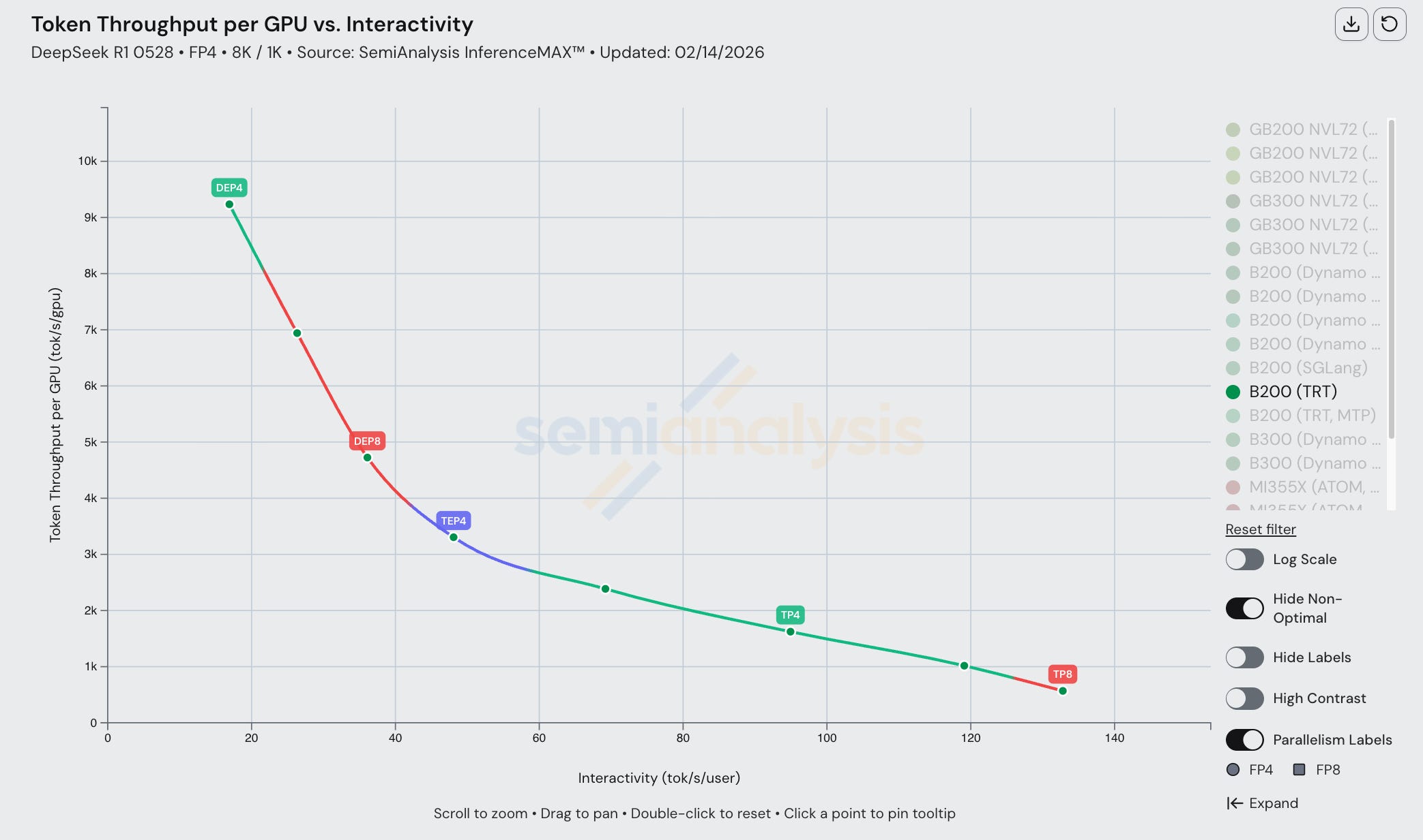
It helps to first understand what parallelism strategies fall on what parts of the Pareto frontier for single-node configurations. Take the example of DeepSeek R1 FP4 8k/1k on a single 8-GPU B200 node with TRT-LLM. The optimal strategy shifts as you move along the frontier, driven primarily by batch size and its effect on expert activation density.
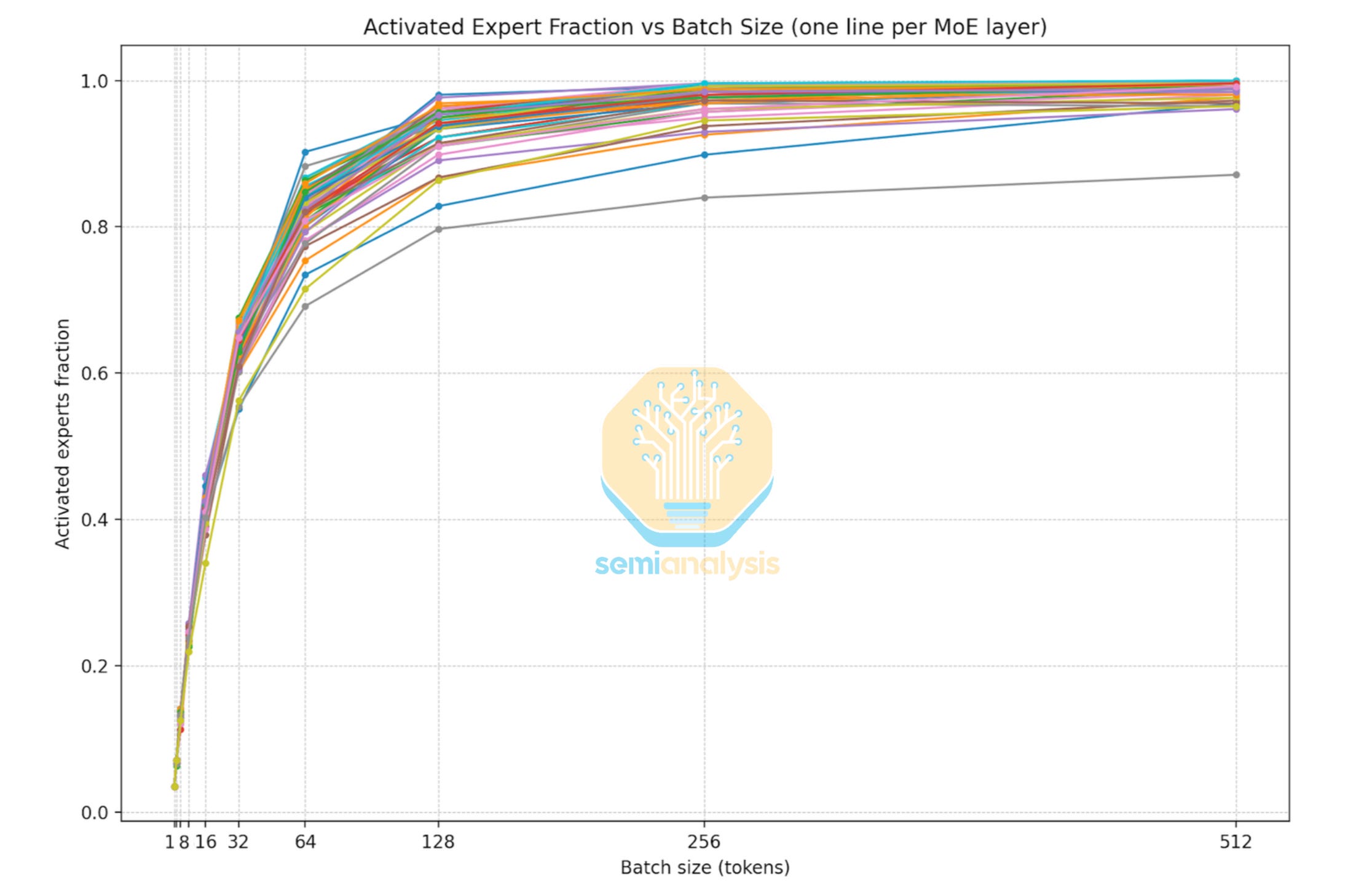
At the highest interactivity levels (batch 1-16), pure TP outperforms any configuration involving EP. At low batch sizes, only a small fraction of experts activate per step. With EP, these activations are distributed unevenly across GPUs: at batch 4, only 32 of 256 experts fire, and any given GPU has roughly a low double digit percent chance of receiving zero routed tokens in a given layer. TP avoids this by sharding every expert across all GPUs, so all 8 GPUs participate equally in every expert computation regardless of which experts the router selects. We collected expert activation ratio versus batch size data while profiling DeepSeek R1, which confirms that at batch sizes 16 and below, expert activation per layer is very low.
As we move to slightly lower interactivities, batch sizes remain small enough that expert weights are still sharded via TP rather than EP. The crossover occurs around batch 32, where approximately 50-60% of experts activate per layer. At this density, EP’s load imbalance becomes tolerable and its token-routing overhead is cheaper than the per-expert all-reduce required by TP. Configurations in this range use TEP: tensor parallelism for attention (all GPUs collaborate on each attention computation), expert parallelism for MoE layers (experts assigned to specific GPUs with all-to-all routing). In the highest throughput, lowest interactivity region of the frontier, batch sizes are large (128+) and configurations shift to full DEP: attention weights are fully replicated across all GPUs as independent data-parallel ranks, experts are distributed via EP, and batch capacity is maximized at the cost of per-token latency. (128+) and attention weights are fully replicated across all DP ranks, maximizing throughput.
We observe the same general pattern when extending to wide EP with disaggregated prefill. Prefill and decode run with separate parallelism strategies and node counts, both tuned to the workload and target interactivity level. Take an 8k/1k workload (prefill heavy) at the high-throughput, low-interactivity end of the frontier. Prefill is the bottleneck as each request requires a forward pass of 8192 input tokens, which is computationally expensive. Recipes in this region allocate more prefill nodes than decode (4P1D, 7P2D, 4P3D) to sustain high prefill throughput. These prefill nodes run DEP configurations, replicating attention weights across independent data-parallel ranks so that multiple long-context prefills can be processed simultaneously. Decode nodes are fewer but run wide DEP with large batch sizes by the same principle as with single node.
On the low interactivity end of the frontier, there are fewer concurrent requests in flight, so a single prefill instance can keep pace with incoming demand. Yet each request still requires 1024 decode steps, and at high interactivity those steps must be fast. Recipes in this region shift to more decode nodes than prefill (1P3D, 1P4D), with each decode instance running TEP at low batch size. Tensor parallelism on attention minimizes per-step latency by sharding the computation across all GPUs in the instance, while expert parallelism handles MoE routing at the moderate batch sizes where EP load balance is sufficient. Multiple small-batch decode instances, rather than fewer large-batch ones, keep per-token latency low while still providing enough concurrent serving capacity.


Dive into DeepSeek R1 Single Node Results
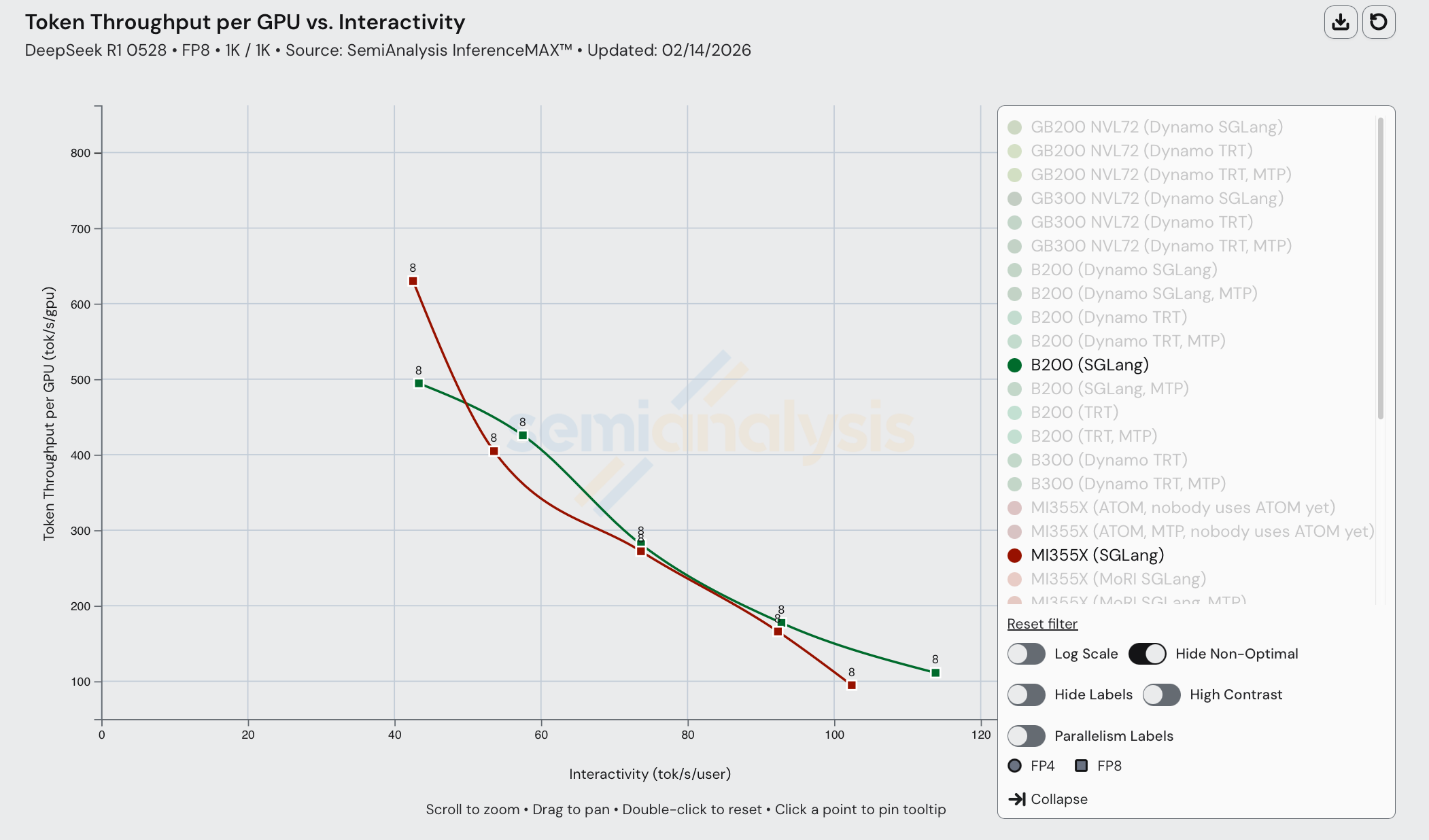
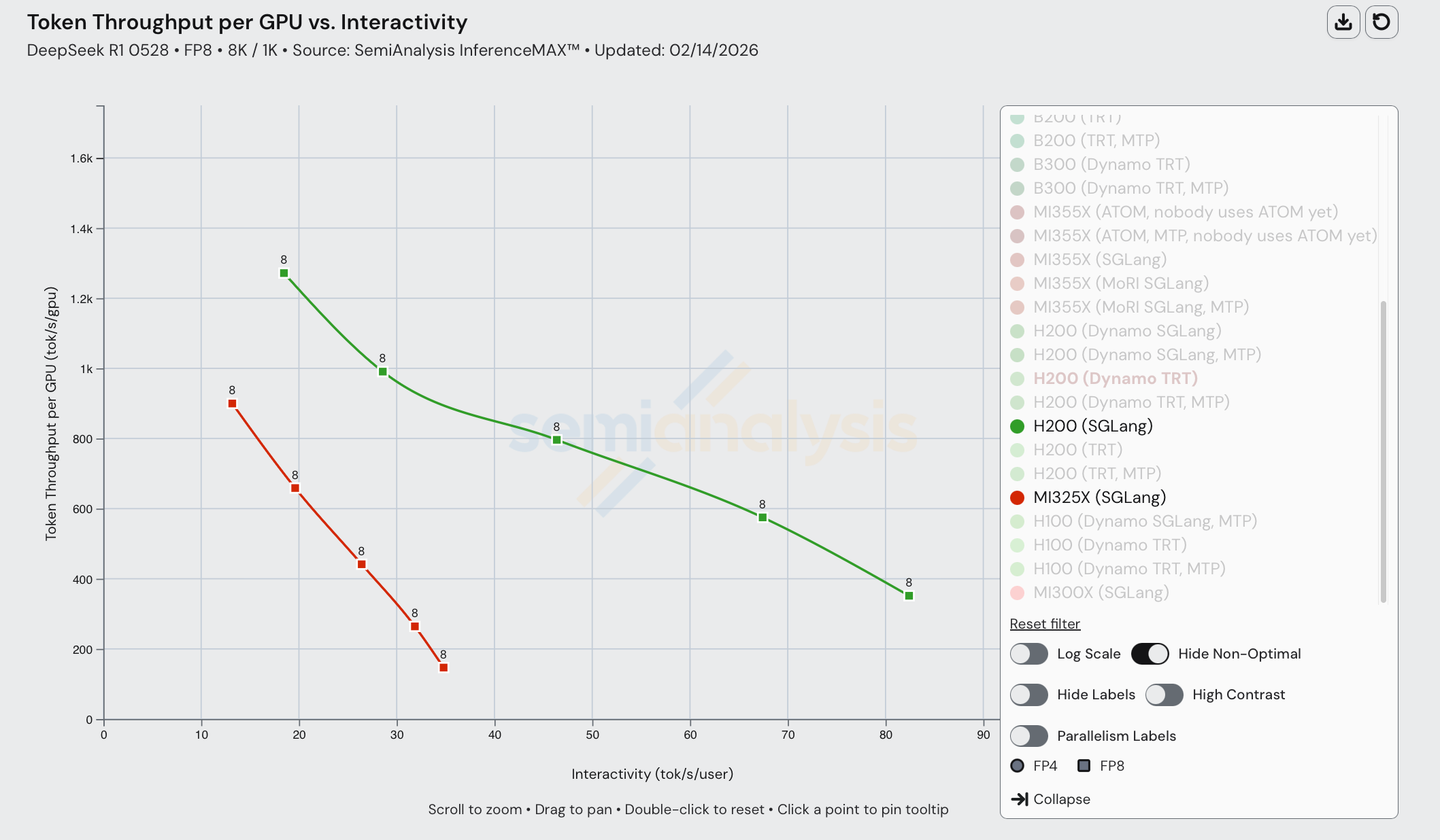
On DeepSeek R1 FP8 1k1k, we see that MI355X is competitive with its counterpart B200 on single node scenarios, despite getting mogged on FP4 multi node scenarios. MI355X (SGLang) even beats B200 (SGLang) in throughput performance at lower interactivity levels. Moreover, MI355X (SGLang) beats B200 (TRT and SGLang) in most cases from a perf/TCO perspective.
Unfortunately, the year is 2026, and most frontier labs and inference providers are not running FP8 nor single node inference.
This result goes to show that AMDs chips are great and can be extremely competitive with Nvidia if only they could move faster on the software front. Speed is the moat.
To that end, we see MI355X fall well behind B200 in performance on FP4:
In comparing DeepSeek R1 FP8 perf between H200 (SGLang) and MI325X (SGLang), not much has changed since our initial release of InferenceXv1 last October. The MI325X data was captured on Feb 12th, 2026 with SGLang 0.5.8 whereas the B200 data was captured Jan 23, 2026 with SGLang 0.5.7.
One thing we note is the considerably smaller interactivity range for MI325X than H200, with H200 ranging from 30-90 tok/sec/user whereas MI325X ranges from only 13-35 tok/sec/user. This is problematic for providers who would like to serve users at a broader range of interactivity.
GPT-OSS 120B Single Node
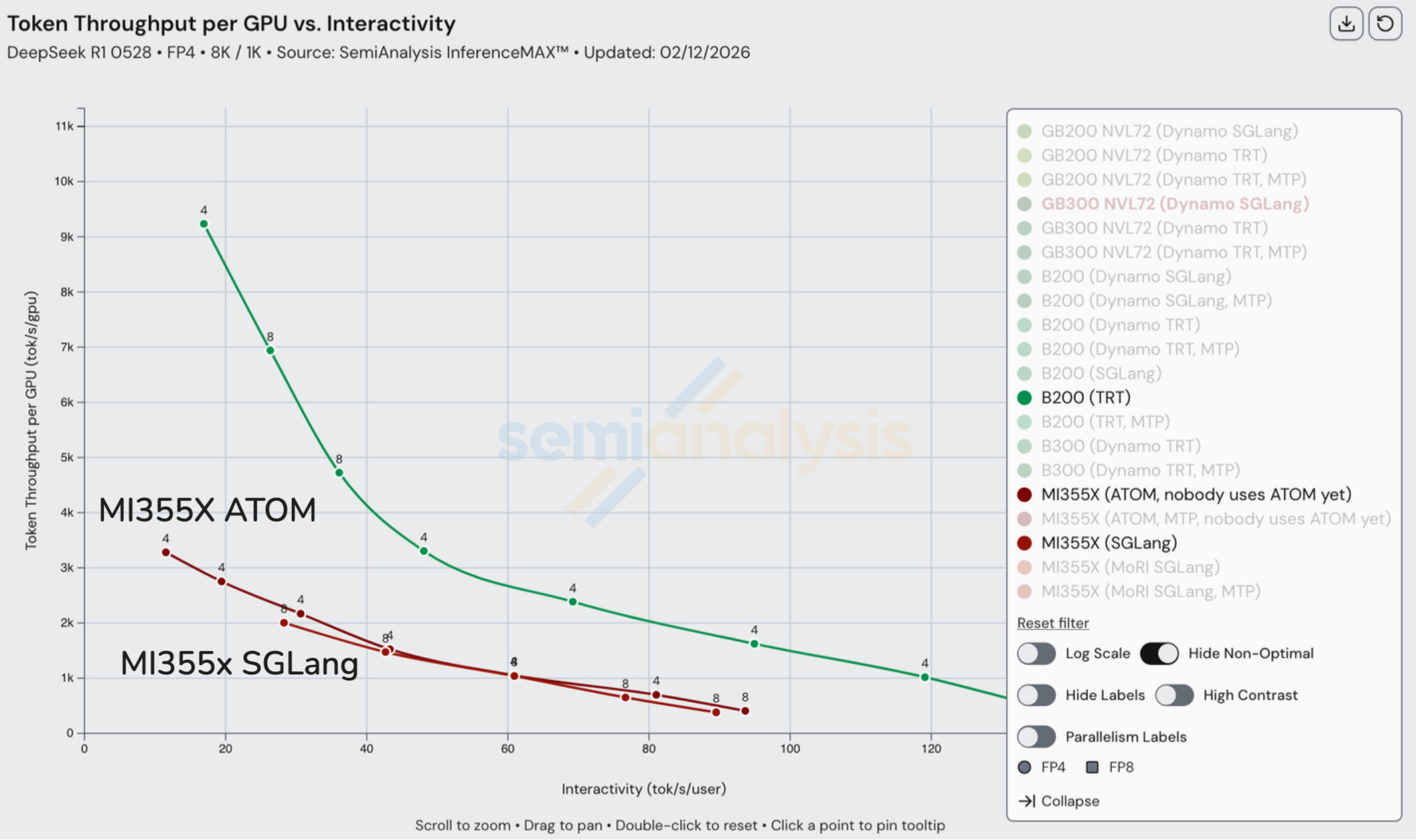
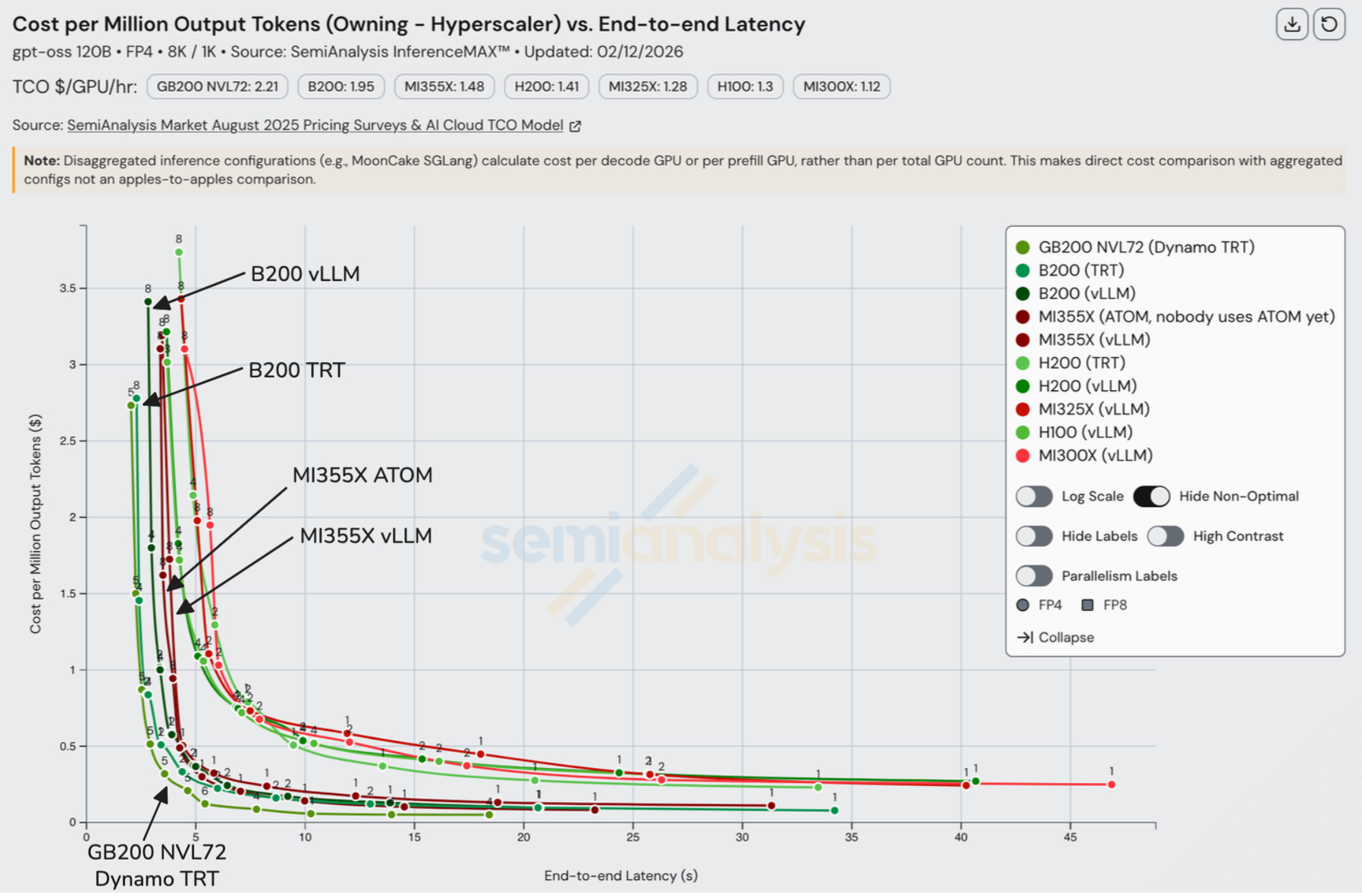
MI300X, MI325X, H200, and H100 group in the lower-left of the throughput vs interactivity plot, indicating broadly similar tradeoffs, with Nvidia generally holding a modest lead. The next step up is MI355X, which delivers roughly more than 2x higher token throughput per GPU at a given interactivity level, relative to that first group. Within MI355X, ATOM shifts the curve toward higher throughput at low interactivity, suggesting it prioritizes peak throughput over per-user responsiveness.
Above that tier sits NVIDIA’s B200 and GB200, which outperform MI355X across the frontier. While B200 and GB200 share the same Blackwell compute die, GB200 achieves a higher throughput–interactivity curve because the platform and serving stack reduce non-compute bottlenecks at scale (interconnect/topology, CPU-GPU coupling, and runtime scheduling), translating into effective scale-out and less overhead per token.
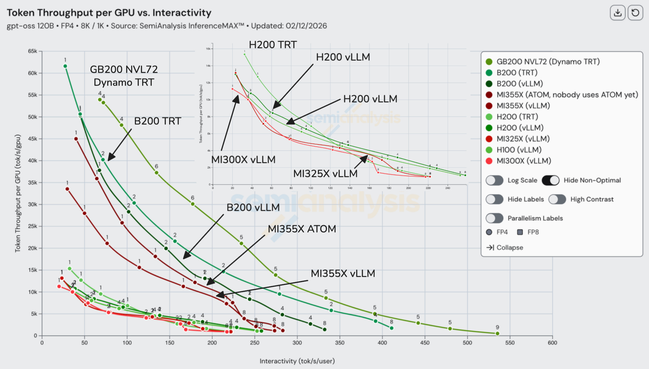
If we add cost into the equation, MI355x becomes more competitive: beating B200 at high throughputs. However, GB200 still takes the cake for being the cheapest choice.
Turning again to the comparison between B200 and GB200 NVL72, it is obvious the impact NVL72 has. We discussed the impact of the GB200 NVL72’s larger 72 GPU scale-up world size vs the B200’s 8 GPU scale-up world size earlier in this article. The output token throughput per GPU more than doubles in the ~100 tok/s/user interactivity range, showing the impact of the NVL72’s larger scale up domain.
Core InferenceX Repo Updates
We have made a few core architectural changes to the InferenceX repository to make it easier to understand and reproduce benchmarks. Additionally, we have fully subscribed to AI usage to maximize productivity and increase developer velocity.
Core Changes Since InferenceXv1
One of the main changes we have made since v1 is the cadence with which we perform sweeps. Previously, we were jestermaxing and performed a full sweep over each configuration nightly. However, as we added more chips, disaggregated prefill, wide EP, and other features, we realized that running every single night was way too time consuming and wasteful. Moreover, it’s just not necessary – benchmarks only really need to be re-run when recipes change or a new software version is released.
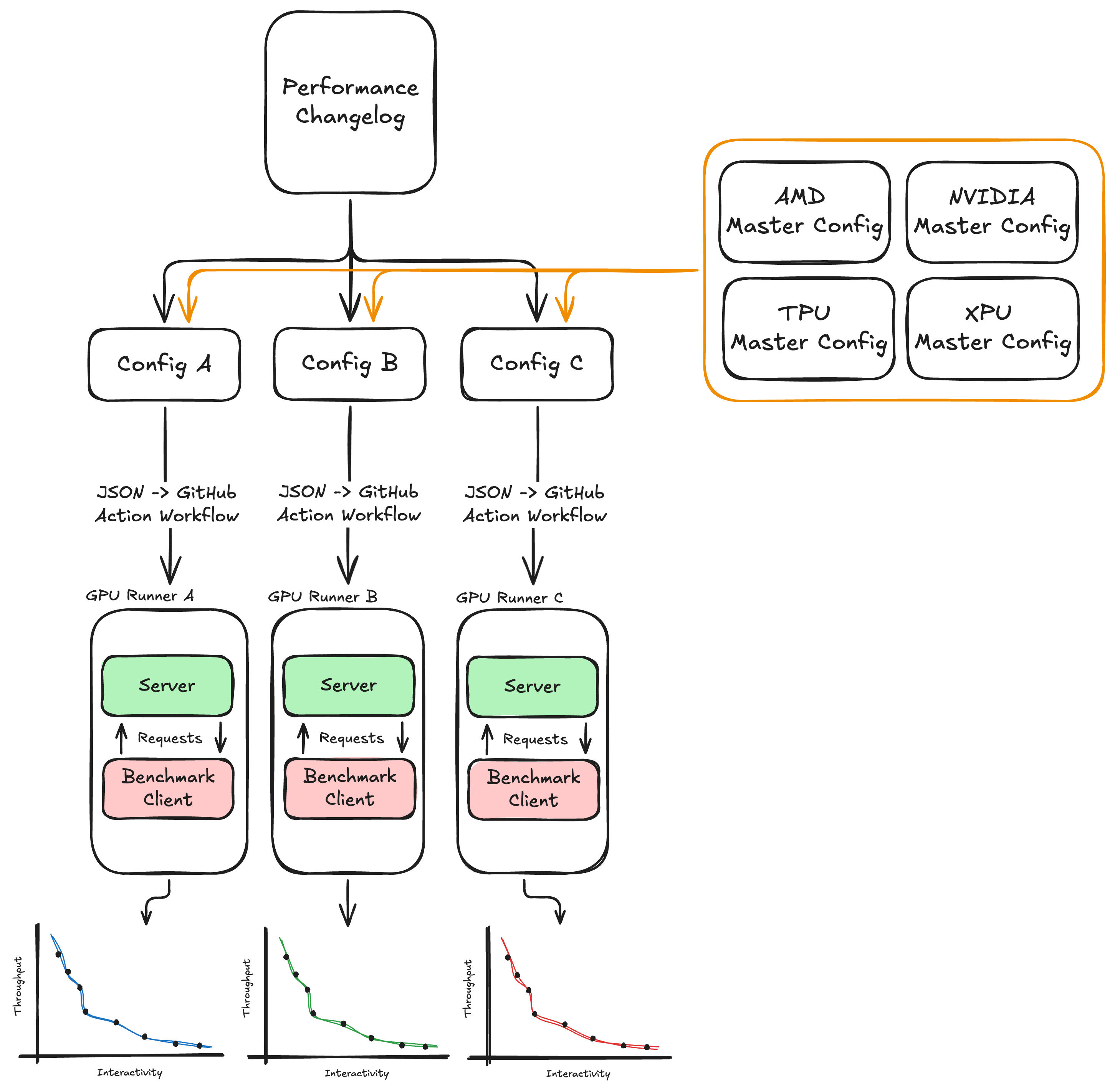
We now trigger sweeps based on additions to a changelog at the root of the repo. When a developer makes a performance-impacting change to a given config, they add an entry to the changelog listing the affected config along with a brief description of the change. All configs are defined in a master configuration YAML file, which serves as the stateful representation of every data point to be swept, including core settings like ISL/OSL, EP, TP, DP, MTP, and so on. When a PR containing a changelog addition is merged, a workflow parses the referenced config keys, pulls the corresponding sweep definitions from the master config, and fans them out as individual GitHub Actions jobs. The jobs collect all data points for the full sweep and upload the results as artifacts.
Below is a high-level diagram of how InferenceX launches jobs.
Klaud Cold AI Usage
Shortly after the release of InferenceX v1, we realized how much developer throughput was being left on the table by not utilizing AI more in our InferenceX development. So, we rolled our sleeves up and decided to embrace Claude Code and begin absorbing intelligence, one token at a time to the point that we are currently spending at a $6,000/day run rate. If you want to contribute towards our KPI of absorbing an annualized $3 million dollars’ worth of Claude intelligence, apply here to join the mission. We started our enlightenment journey when we realized the GitHub Copilot agent was free – at first we couldn’t believe this feature came at no cost! We soon realized that Copilot is terrible and it became apparent why GitHub was giving it away for free. You probably would have had to pay us to keep using it.
We had been using Claude Code locally ever since it was released. But recently, we have integrated Claude Code into InferenceX development, using it for the usual tasks such as reviewing PRs, but we also have given it the ability to perform sweeps on clusters. With the workflows we setup, Claude can manually initiate runs, view the results, and iterate. This has enabled us to deploy quick fixes easily on the go via the GitHub app.
Another cool use case is using Claude to find recipes for new vLLM/SGLang images. When a new image is released, recipes sometimes need to be updated to achieve optimal performance (new environment variables, modified engine arguments, etc.) With our Claude Code integration, we simply open an issue and ask Claude to search through all commits in the image changelog to find necessary changes to be added to the recipe. This works quite well, and although it’s not perfect, it often gives a good starting point.
GitHub Actions
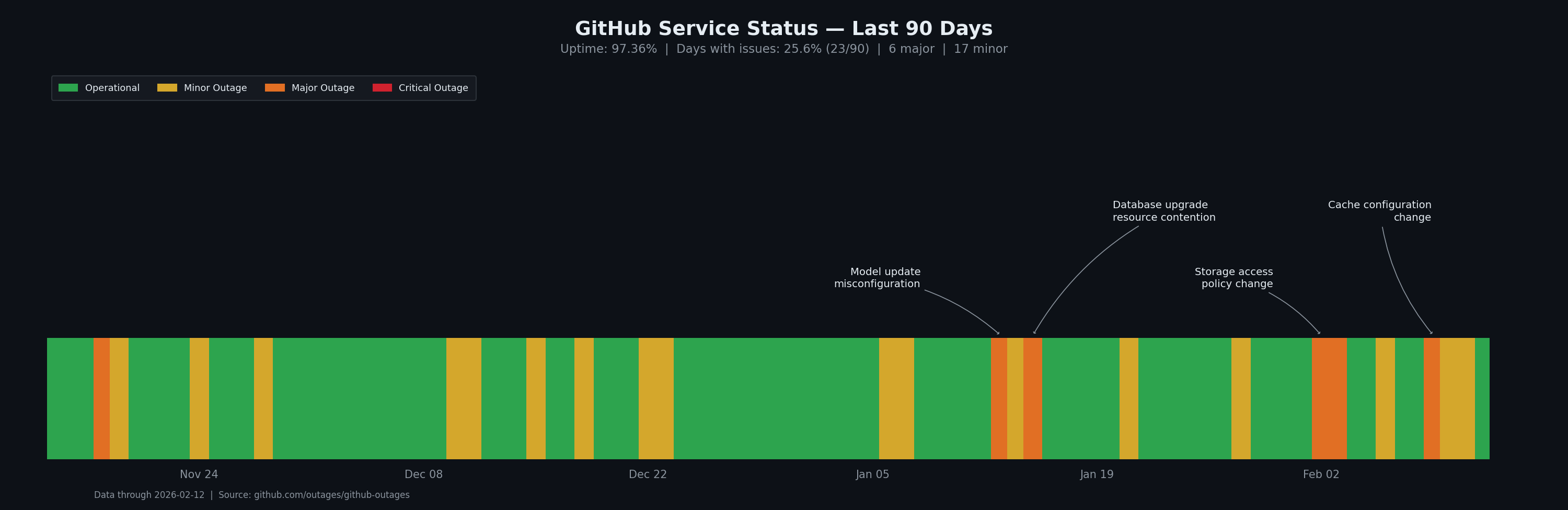
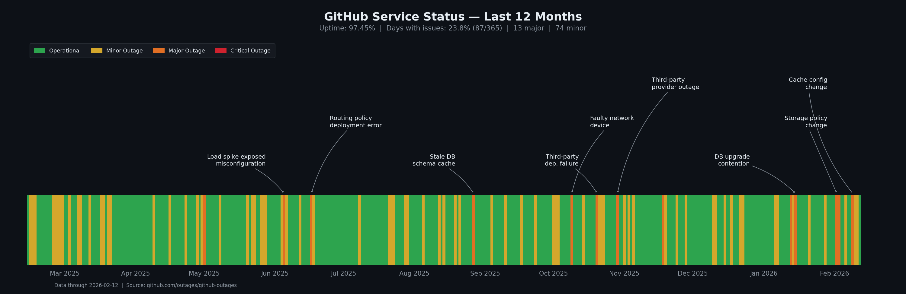
In the spirit of open source, all runs occur on GitHub Actions, so benchmark results are verifiable, transparent, and reproducible. However, GitHub outages have been a constant obstacle to our goals recently. We have seen more unicorns lately than any other animal! But maybe it’s time for us to touch some grass.
Microsoft/GitHub themselves are aware of this and have stopped updating its status page with aggregate uptime numbers and are down to a single 9: 97.36% over the past 90 days. The problem doesn’t seem to go away if you choose to ignore it...
All in all, GitHub Actions is just alright. It provides a painfully average experience for developers. It is certainly not meant for launching thousands of jobs across a fleet of hundreds of GPUs. Nevertheless, we have worked closely with some GitHub Actions engineers since our launch to better meet the needs of InferenceX, and we can confidently say they have been a pleasure to work with. Moreover, one of our direct asks was to implement lazy loading for jobs when clicking on a workflow run and, while it did take them a while, they eventually implemented the feature.
Future of InferenceX
Since the initial release of InferenceX in early October 2025, we have worked hard to continuously improve InferenceX. After release, we spent some time refactoring the codebase to make it more scalable, such that new models and inference techniques can now be added in a “plug and play” fashion. These changes enabled us to seamlessly integrate PD-disagg benchmarks for H100, H200, B200, B300, GB200, GB300, and MI355X. We also added accuracy evaluations to our default benchmark pipeline to ensure visibility into model performance across all configurations.
Although we have made many improvements since our release, there is still much work to be done to achieve the north star goal of providing the most real-world inference benchmarks possible. To achieve this goal, we plan to benchmark on real datasets, add an agentic coding performance benchmark, include more SOTA inference optimizations, benchmark more models, and so much more.
Migration to Multi Turn Real Multi-Turn Chat and Agentic Coding Datasets
Currently, InferenceX uses completely random tokens as input for benchmarking. We then vary the ISL/OSL uniformly subject to the distribution [ISL*0.8, ISL], similarly for OSL. Because of the random data, we disable prefix caching in all our benchmarks, as the expected value of a prefix cache hit rate on completely random data is 0%. Furthermore, all the random data is single-turn, meaning each conversation contains only one prompt and one response. While this provides a good baseline Pareto frontier, it is not a practical benchmark setup that mimics real-world production inference workloads.
In the near term, we will create a basic multi-turn benchmark with a dataset like allenai/WildChat-4.8M, which captures real users’ multi-turn conversations. In addition to enabling prefix caching on all scenarios, we will enable KV cache CPU offloading, as this is what we see being done in production workloads. This will more accurately evaluate the strengths and weaknesses of each chip. For instance, MI355X has 288GB HBM3e versus B200s 192GB. Therefore, we expect MI355X to perform better in a high concurrency multiturn scenarios as more memory can be allocated to the KV cache. On the other hand, in scenarios where the GPU KV cache is stressed and blocks are offloaded to the CPU, we expect the GBs to excel as these chips have 900GB/s bidirectional CPU-GPU bandwidth, compared to 128GB/s / 256GB/s on HGX with PCIe 5.0 and 6.0, respectively. Moreover, currently we see AMD’s software for CPU offloading is poor, which may negatively affect performance in the same scenarios.
The point is: real-world multiturn datasets test more SOTA inference engine features and can capture more nuanced and robust performance data across all chips.
With the rise of Claude Code, Codex, and Kimi, it is becoming increasingly important to benchmark performance in agentic coding scenarios. Like above, these scenarios are multi-turn but also include extremely long context conversations as well as tool use. In the next few months, we plan on creating a benchmark suite that will most accurately capture the performance of open models in these agentic coding scenarios across all chips.
Adding TPU, Trainium and More Models
Currently, we continuously benchmark DeepSeek R1 and GPT OSS 120B (previously Llama 3.1 70B as well). To keep up with the newest model architectures, we plan on adding DeepSeek V3.2 (w/ DSA), DeepSeek V4 on Day 0, Kimi K2.5, Qwen3, GLM5, and many more over the course of the next few months. We will also eventually add multi-modal models and be using EPD & CFD (invented by TogetherAI) optimization too.
In addition to new models, we are actively working on adding both TPU and Trainium.