

RL Systems Mind the Gap: Matching Trainer and Generator Throughput
RL Training Infrastructure, GRPO, PipelineRL, Async RL, Policy Staleness, RL Sandbox Infra, CPU Requirements, TCO Analysis, Thinking Machines Tinker
The Cost of Capability
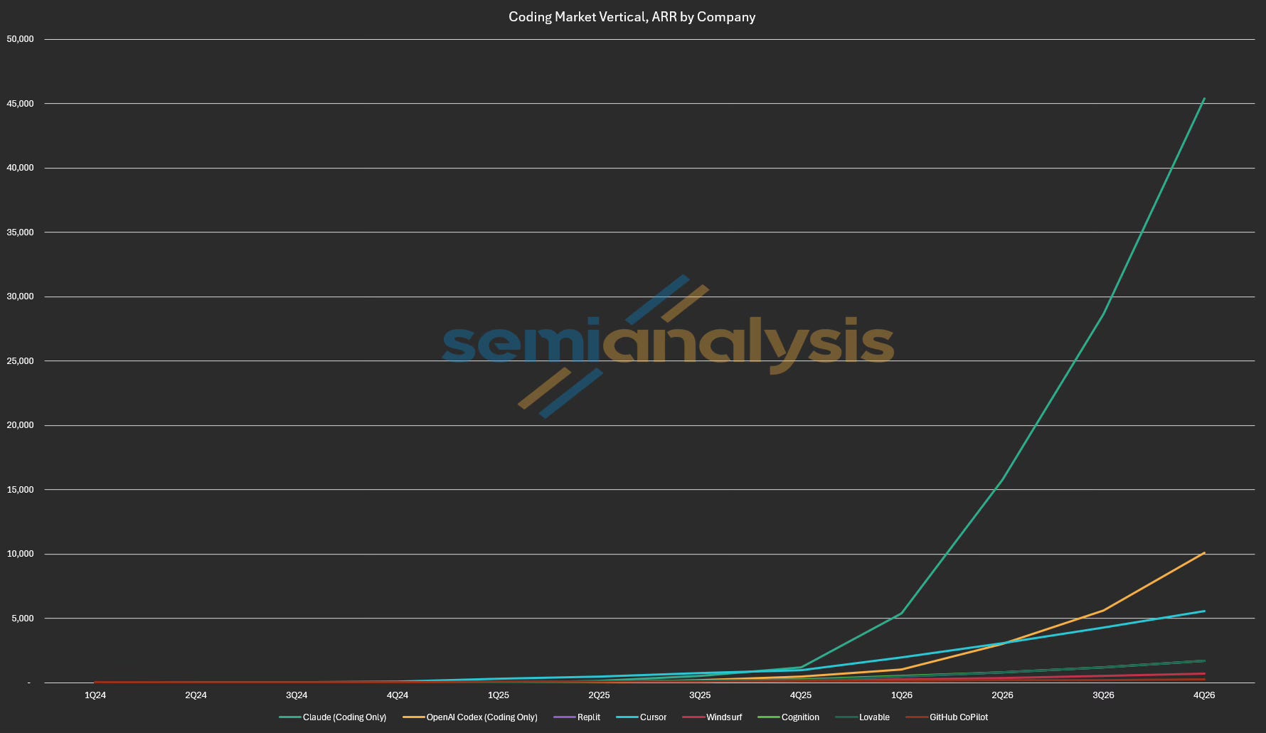
Coding assistants are the greatest B2B SaaS application the world has ever seen: a $30B+ ARR market across the six largest players today, on track to clear $100B by year end, per our tokenomics model.
The agentic coding capabilities of those assistants don’t come from pre-training alone. Post-training, and reinforcement learning (RL) in particular, is what elicits these capabilities from such pre-trained models. Concretely, Claude Opus 4.8 scores 69.2% on SWE-bench Pro and 74.6% on Terminal-Bench 2.1, and RL training is a major part of what drives the score.
Dario Amodei, Anthropic’s CEO, has described RL as showing the same kind of scaling pre-training once did, where performance climbs log-linearly with how long you train (link). However, that scaling is enormously expensive, which makes RL system efficiency critical: it sets how much RL you can afford, and with it how far model capabilities can go.
What governs the efficiency of an RL training system? In this article, we conducted RL training experiments on open models with open-source RL frameworks, and compared pricing to hosted RL training solutions such as Tinker. We show that system efficiency comes down to matching trainer and generator throughput.
Acknowledgements
We’d like to thank the following for close collaboration:
Prime Intellect: Matej Sirovatka, Ameen Patel, Sami Jaghouar, Johannes Hagemann. We thank their help with providing recipes, hardware resources, and article feedback
Modal: Peyton Walters, Nan Jiang, Erik Dunteman. We also thank Modal’s API credit sponsorship
vLLM / Inferact: Kaichao You, Ao Shen
verl developers: Xibin Wu, Yuyang Ding, Yan Bai
slime developers
Verda: Provided compute for experiments
We’d also like to thank the following for reviewing and offering feedback:
Linden Li, Applied Compute: Gave great advice, and whose AIE talk inspired the article
Periodic Labs: Dennis van der Staay, Byron Hsu
Randy Ardywibowo, Perplexity AI
λux, Non-Euclidean Pasture
Simon Guo, Thinking Machines Lab
The Three Actors
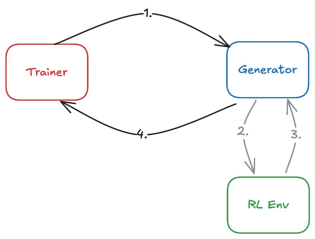
An open-source RL training system has three actors: the generator, the RL environment, and the trainer. The generator performs inference on prompts from the dataset, generating a rollout: a prompt and a model’s generated response. Unlike in pre-training, the dataset only provides prompts, not the full target. Instead, the system generates the training signal. To generate rollouts, the generator interacts with the RL environment. The RL environment produces a reward based on the rollout. For example, a code environment executes the generated code in a sandbox and gives reward scores based on the test case pass rate. Then, the trainer ingests rollouts and rewards generated by the generator and trains the model, producing new model weights. Finally, the trainer pushes the new weights to the generator, closing the loop of an RL training step.
The RL Algorithm, Just Enough
Unlike pre-training, which maximizes the log-likelihood, RL training maximizes the expected reward. Group-Relative Policy Optimization (GRPO) is the open-source standard, and most open-weight models train with some variant of it.
GRPO samples multiple completions for each prompt, forming a group of rollouts. We assign each rollout a reward, a score of the rollout. We then compute each rollout’s advantage: its reward relative to the group’s average, capturing how much better or worse it did than a typical rollout for that prompt. Rollouts above the group average get reinforced, and those below get suppressed.
If every rollout in a group gets the same reward, each one equals the group average, so every advantage is zero and the group produces no training signal. This is governed by the group’s reward distribution: a group only teaches the model something when its rollouts show different behaviors. The extreme case is a uniform distribution, which happens when a task is too easy (every rollout passes) or too hard (every rollout fails), i.e. when the solve rate is near 100% or near 0%.
From Synchronous to Asynchronous RL
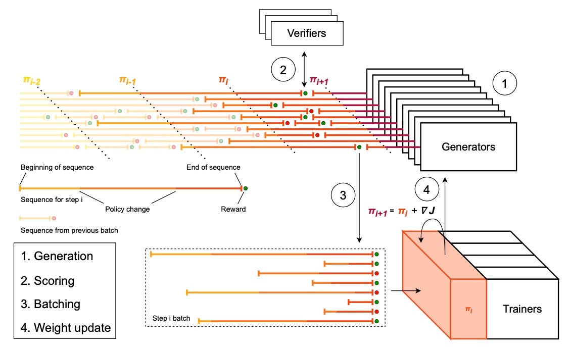
Classic policy gradient algorithms (which GRPO is based upon) assume the rollouts in a group come from the same policy, i.e., the model with the same set of weights. In the context of the training system, this means the generator cannot update weights until it finishes the current batch of rollouts. As a result, if the trainer finishes a training step, it’ll have to wait for the generator. This leads to synchronous execution of training and generation, greatly reducing system efficiency.
PipelineRL introduces asynchrony into the system by allowing the trainer to push new weights to the generator while rollouts are still in progress (in-flight weight updates). This way, the trainer can overlap its execution with the generator’s rollout. However, this comes with a cost. A sample, the unit a trainer consumes, is defined as a rollout and the reward the RL environment assigned to it. With in-flight weight updates, each sample is generated by a mixture of old and new policies. We refer to the phenomenon as policy staleness.
PipelineRL shows that RL algorithms can tolerate policy staleness to an extent. Samples too stale degrade model learning. Synchronous execution wastes too much compute to be practical at scale, and async techniques are essential. In effect, PipelineRL is a throughput-matching scheme with bounded policy staleness. It allows the trainer and generator to run at different speeds, capped by how stale samples can get. This is why PipelineRL has become the de facto implementation in open-source RL training.
The RL Environment and Sandbox
The RL environment provides feedback to the model for the model to learn how to do a task. Practically, the RL environment is implemented as a sandbox, a containerized runtime for code execution. Depending on the complexity of the RL environment, it could range from lightweight Firecracker micro-VMs (micro-Virtual Machines) to full-blown QEMU VMs.
Sandboxes for RL environments have unique system challenges. The interaction latency between the generator and the RL environment is critical to the end-to-end rollout latency, and sandbox startup latency is one of the major overheads. Sandbox service companies like Modal optimize the startup latency with techniques like content-addressed caching.
Serving at scale is also challenging: sandboxes scale along with the number of concurrent rollouts, and the number of live sandboxes fluctuates greatly as rollouts are pruned or completed.
Finally, sandboxes need to be robust against system failures. During learning, a model’s unexpected behaviors may deplete a sandbox’s designated resources. For instance, creating a million files can cause the sandbox to run out of memory. Sandbox orchestration needs to be able to detect and recover from those system failures.
The Throughput-Matching Framework
Quantifying Trainer and Generator Throughput
We view the RL training system as a queue: the generator produces rollouts into a queue, and the trainer consumes from it. When the generator is slower than the trainer, the queue empties and the trainer starves, idling between steps. When the generator is faster, the queue grows and its samples age, causing policy staleness issues.
We model the system efficiency through the lens of matching the producer (generator) and consumer (trainer) throughputs. In an ideal RL training system, the trainer consumption rate should be roughly equal to the generator production rate. The trainer consumes samples, performs a training step, and then broadcasts weights to the generator. We measure the training step time, including the idle time waiting for new samples, the compute time, and the weight broadcast time. We further derive the sample throughput (samples / compute time) to represent the trainer consumption rate. We also calculate FLOP/s per GPU and model FLOPs utilization (MFU) to characterize hardware efficiency.
The generator produces samples through LLM inference and RL environment interactions. Since the straggler, the longest rollout in a group, sets the group's completion time, we measure end-to-end latency to estimate the average sample throughput. We can derive the sample throughput (samples / end-to-end latency) to represent the generator production rate.
We further break down the latency into LLM inference time and RL environment interaction time. RL environment interaction involves sandbox startup latency and sandbox execution time.
Throughput Constraints
Multiple factors constrain the upper and lower bound of the throughput. The trainer consumption rate is samples per step / training step time.
Factors that affect the number of samples include:
Group size: N samples per prompt, N is usually 8 or 16. Depending on the task difficulty, we increase N to strengthen the advantage signal, e.g., setting N=64 for GPU kernel writing tasks. Larger groups increase the samples per step
Reward distribution and advantage filtering: Reward distribution of a rollout group affects the sample advantage, and it reduces the samples per step under different advantage filtering strategies. For example, task difficulty: Tasks being too easy or too hard leads to uniform reward distribution (All zero or all full rewards), causing zero advantage. If we drop zero-advantage samples, it reduces the samples per step.
Batch size: There’s a minimum effective batch size that enables stable learning. We typically deploy the trainer on sufficient GPU nodes to hold those batches
Factors that affect the training step time include:
Model: Model architecture, including model size, activation size, model precision, dictates the memory usage, setting a minimum GPU count to perform forward and backward pass without running out of memory. It also determines what operations the GPU executes, affecting the training step time
Parallelism and memory configurations: Tensor/Pipeline/Data/Expert Parallelism, Fully-Sharded Data Parallelism (FSDP), memory offloading, activation checkpointing. They are affected by the GPU count and determine the system efficiency and the training step time
On the generator side, we define the generator production rate as the number of concurrent rollouts / end-to-end latency.
Factors that affect end-to-end latency include:
Inference throughput: Recipe tuning for the inference engine, including parallelism strategies, KV cache quantization, PD disaggregation, and speculative decoding
Sandbox latency: Sandbox startup time and execution time
Reward modeling type: Math and coding tasks may have lightweight verifiers as reward models, while writing tasks may use LLM judges. Reward model types determine the rollout evaluation latency: lightweight verifiers are fast, and LLM judges are comparatively slow
Reward shape: Process Reward Models (PRMs) may evaluate the rollout per turn, whereas some reward models evaluate only the full rollout. This determines the reward assignment latency
Concurrency, or the number of concurrent rollouts, is limited by KV cache memory space and average sequence length. The aggregate memory capacity of generation nodes - model weights and activations are the space for KV cache. KV cache dictates the maximum number of tokens the generator can hold, and dividing it by the average sequence length gives us an estimate of max concurrency.
Not all generated samples are consumed by the trainer due to training signal quality differences. We further define the effective generator production rate as acceptance rate × generator production rate. Factors that affect the acceptance rate include:
Early pruning: We prune rollouts before completion based on heuristic length caps, value functions, or intermediate-result verifier checks. This dynamically reduces the number of concurrent rollouts
Adaptive sampling: We reject rollouts based on criteria, such as online advantage filtering
Policy Staleness
Staleness is the gap between the policy version that produced the sample and the one that the trainer uses when it applies the gradient. Staleness is a byproduct of async training: the trainer pushes weight updates in-flight while rollouts are being generated.
Staleness happens at different granularities. At the trajectory level, staleness is the gap between the policy that the rollout starts generating with and the newer policy the trainer updates, e.g. the trainer is at version t+k while the trajectory started from version t. Token-level staleness occurs when in-flight weight updates happen mid-rollout, so different policy versions generate different parts of a rollout. Policy staleness also happens at an environment state-level, which we explain more in the Partial Rollout and Stateful Sandbox Design section.
Policy staleness means the trainer trains the model on off-policy signals, which can destabilize training, so we typically set a policy staleness budget. The policy staleness budget bounds how stale a sample can be, i.e. how far the generator is allowed to run ahead of the trainer before its samples are rejected. This in turn caps the gap between the generator’s production rate and the trainer’s consumption rate, which is what lets the two run at different speeds.
The policy staleness budget limits the max difference between the trainer consumption rate and the effective generator production rate. Concretely, it limits how many steps the generator can be ahead of the trainer, so the RL algorithm can tolerate the max staleness in samples.
The Moving Target: Model Capability and Behavior
Model capability and behavior are first-class system variables in RL training. Model capability determines how well the model can solve a task, measured by solve rate: what percentage of the rollouts in a group passes the verification. When the solve rate is near 0 or near 100%, the reward distribution is uniform, leading to zero advantage, and collapses the training signal. This drives decisions including group size and advantage filtering strategies. It also shapes the curriculum: the order of tasks being presented to the model. The curriculum is chosen to keep the solve rate at a productive middle band, so the tasks are neither too easy nor too hard for the model’s current capabilities.
A model's token usage behavior affects the output length, which indirectly determines the max concurrent rollouts in the generator. RL training typically elicits Chain-of-Thought reasoning, causing a model to generate long reasoning traces. This behavior drives the average output length, which increases KV cache usage. Under the same memory budget, this reduces the max concurrent rollouts and increases the sample generation end-to-end latency.
A model’s tool call behavior affects the sandbox time in the end-to-end latency. Concretely, more tool calls increase the sandbox time, and unexpected tool call operations strain the sandbox infra. We measure the tool call behavior with the number of tool calls and the sandbox error rate.
Both model capability and behavior shift during RL training. Model capability improves, and behavior drifts. The constraints move with them, and the training system has to adapt to ensure efficiency.
Case Studies
We ran experiments to ground our theory, and we shared our experiences with open-source RL frameworks.
We select the following configurations:
Model: We chose Mixture-of-Experts (MoE) models since SoTA open-source models are mostly MoEs
RL environment and tasks: We chose agentic coding tasks for its popularity and its sandbox workload complexity, allowing us to see sandbox performance characteristics
Node count: We aim for experiments with at least 10 nodes to show the trainer-generator dynamics and fit training MoEs
Long Model Response and Early Exploration Training Phase
Setup
Model: Qwen3-235B-A22B-Thinking-2507. We use BF16 precision for training and the FP8 variant for sample generation, a common setup in RL training
Trainer: 64 H200 GPUs, FSDP, EP8, CPU-offloaded optimizer states and activations
Generator: 192 GPUs, 24 inference instances: Each DP1, TP8, EP8
Batch Size: 512 samples
Group Size: 16 rollouts per problem
Problems per batch: 32 problems
Max sequence length: 32K
Maximum policy staleness: 16 steps
RL environment: Mini SWE Agent Plus, with Prime Intellect Sandboxes
RL framework: Prime RL
Code: Recipe coming soon in repo’s main branch. Original commit here
Analysis
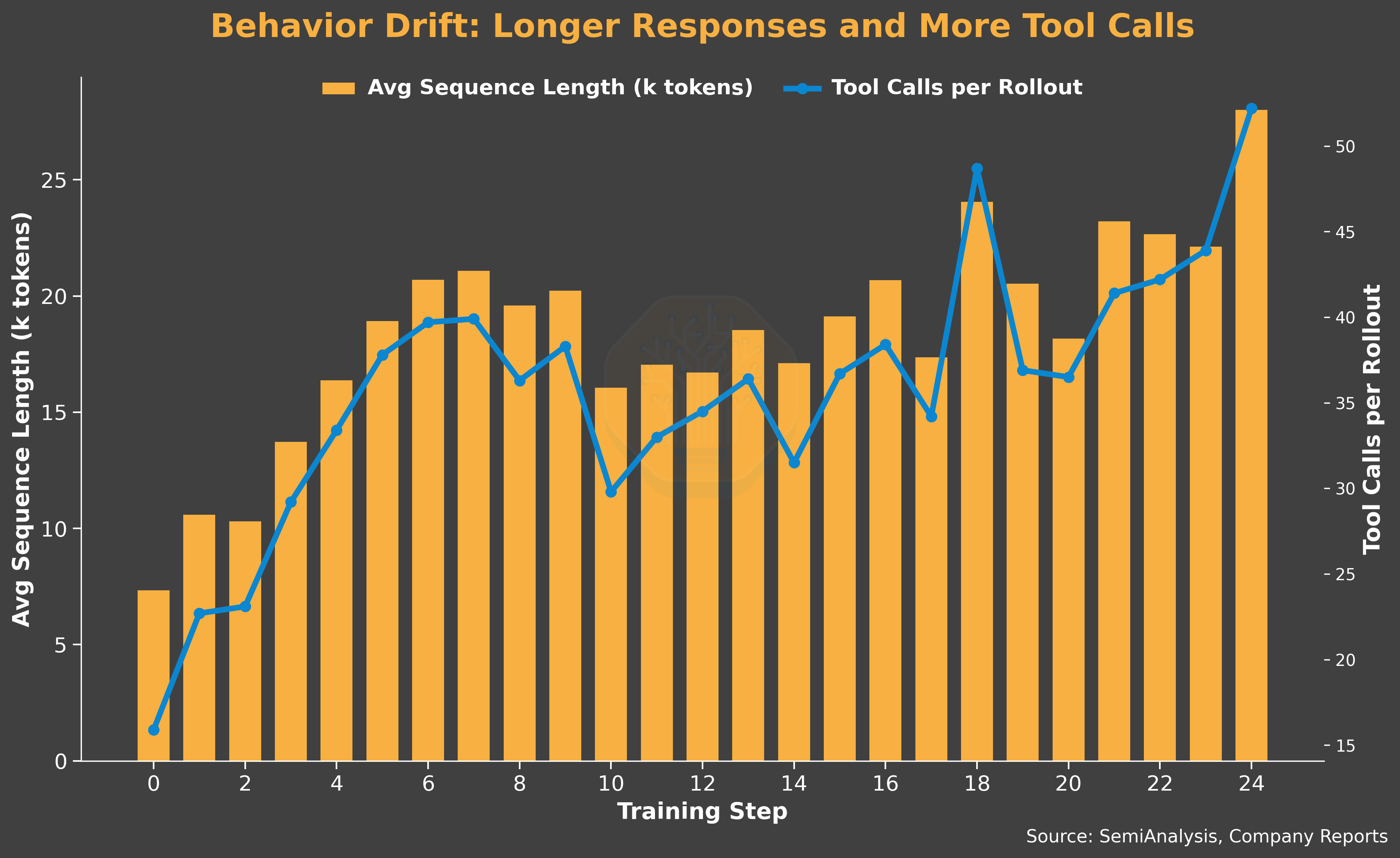
In this case study, we show how two factors influence the system efficiency: how the model produces long responses with long thinking traces, and how well the model learns the task.
The model’s long response behavior is the dominant driver of LLM inference time, which makes up the majority of sample generation time. Long-response variance also drives severe tail latency within each rollout group, which forces a system-side mitigation: oversampling. With oversampling the generator launches more concurrent rollouts than the trainer needs per batch and it discards unfinished or errored ones as soon as the target count is reached. In this run we discard a relatively high 60% of dispatched rollouts, reflecting how skewed the latency distribution becomes when the responses are long.
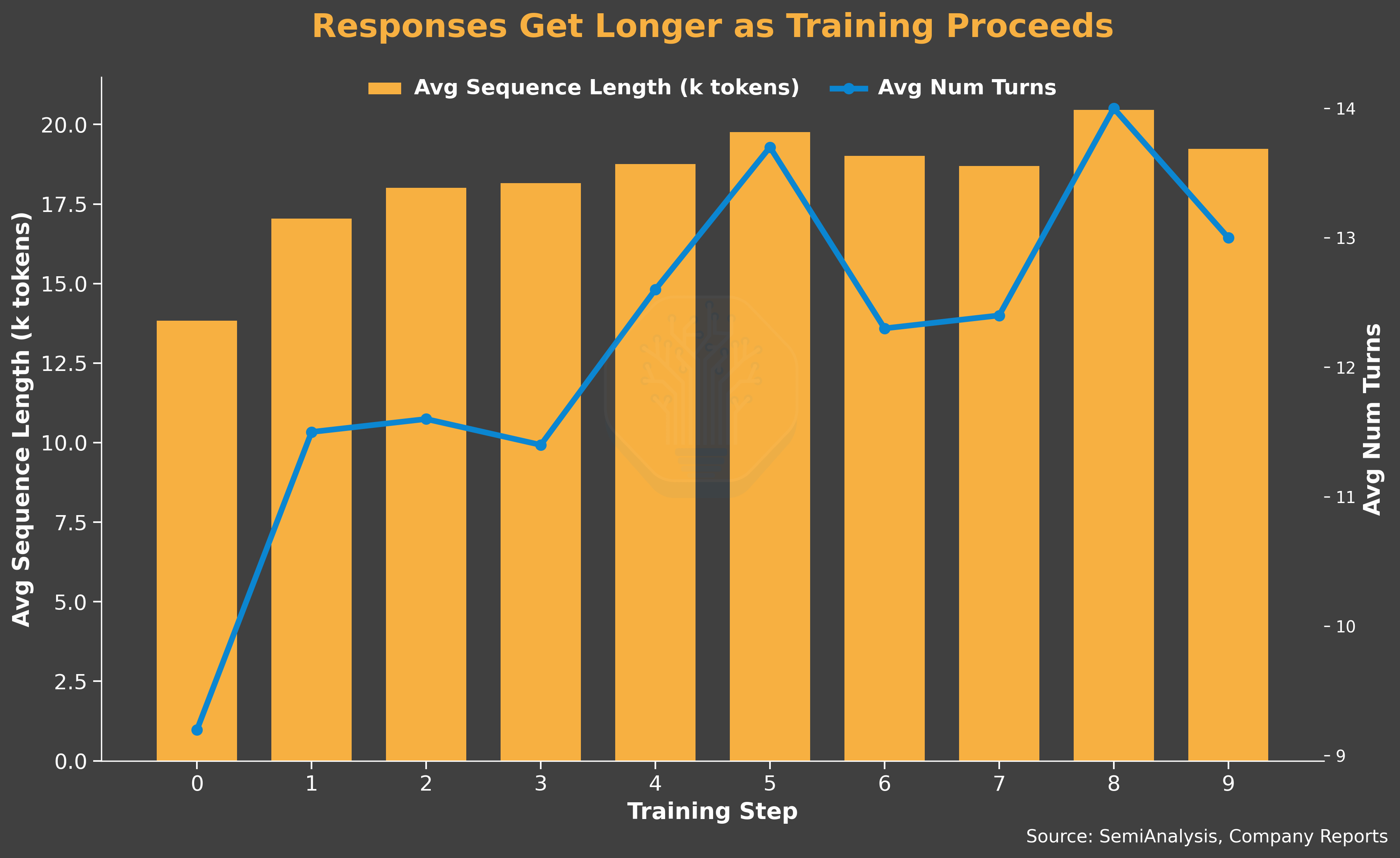
On the model capability side, the curriculum is slightly too hard for the base model. We observe the number of rollout groups that produce zero solutions jump sharply after the first training step, but average reward and pass@16 are slowly recovering. These are signs that the early RL exploration pushed the policy away from previously solvable problems before it could relearn them.
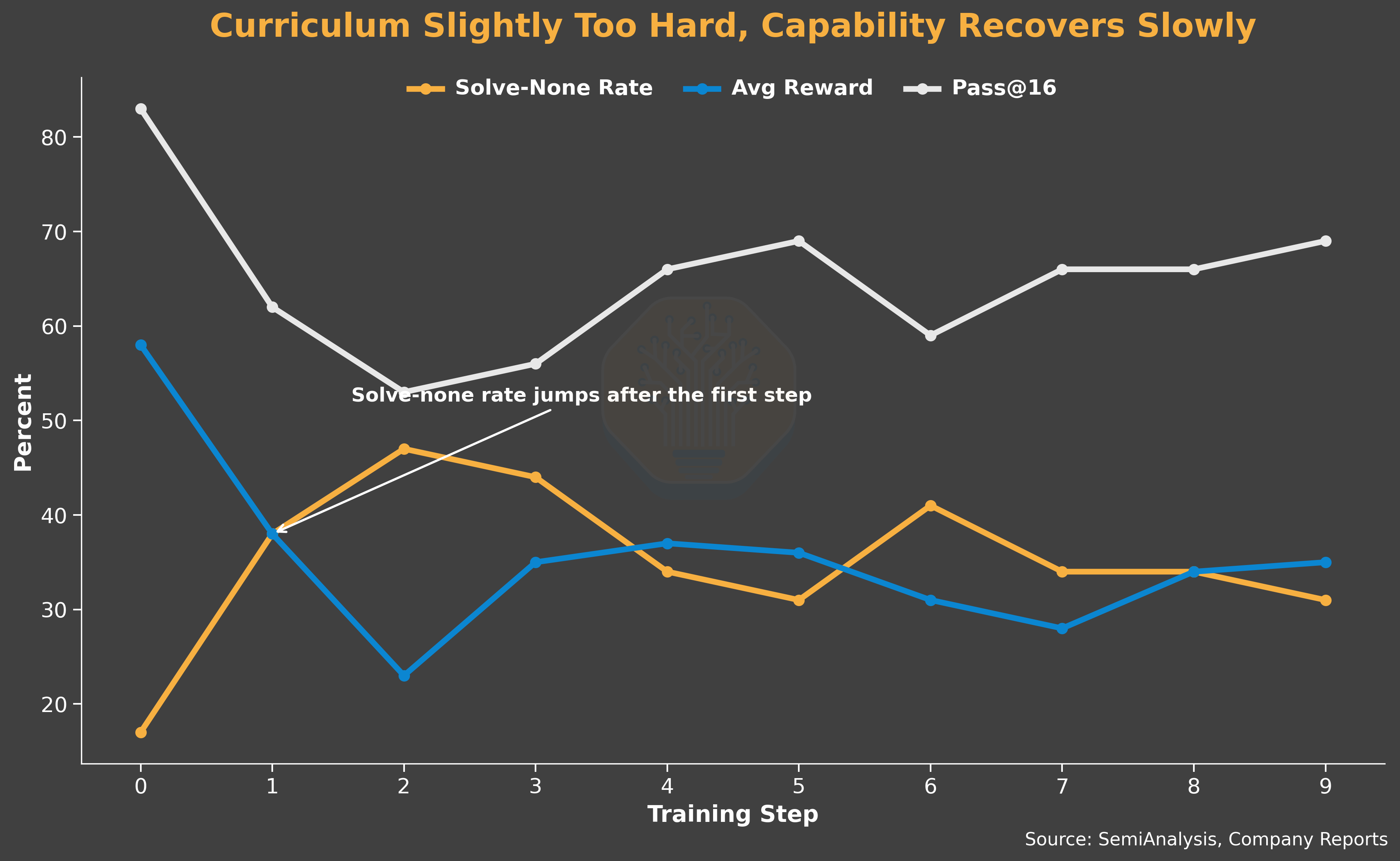
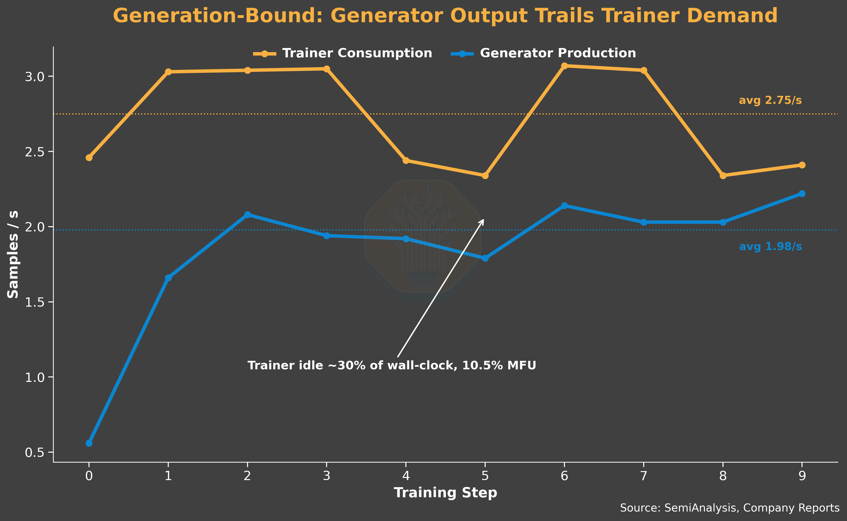
The combined effect is a generation-bound system: the queue runs dry and the trainer starves. To mitigate this issue, we trade off trainer efficiency for generator efficiency. The trainer consumes samples at 2.75 sample/s, waits 30% of the wall-clock time, and runs at 10.5% MFU. On the other hand, the generator delivers 1.95 sample/s and uses 3x the trainer’s compute. This underscores how much inference efficiency matters during RL training.
Frequent Tool Use and Easy Task
Setup
Model: GLM-5. We use BF16 precision for training and the FP8 variant for sample generation
Trainer: 128 H200 GPUs, FSDP, CP2, EP8, CPU-offloaded optimizer states
Generator: 128 H200 GPUs, 2x 64-GPU inference replicas
PD Disaggregation: 32 prefill GPUs, 32 decode GPUs, both DP32 and EP32
1TB KV cache offload per node
Batch Size: 512 samples
Group Size: 16 rollouts per problem
Problems per batch: 32 problems
Max sequence length: 64K
Maximum policy staleness: 16 steps
RL environment: Mini SWE Agent Plus, with Prime Intellect Sandboxes
RL framework: Prime RL
Code: Recipe coming soon in repo’s main branch. Original commit here
Analysis
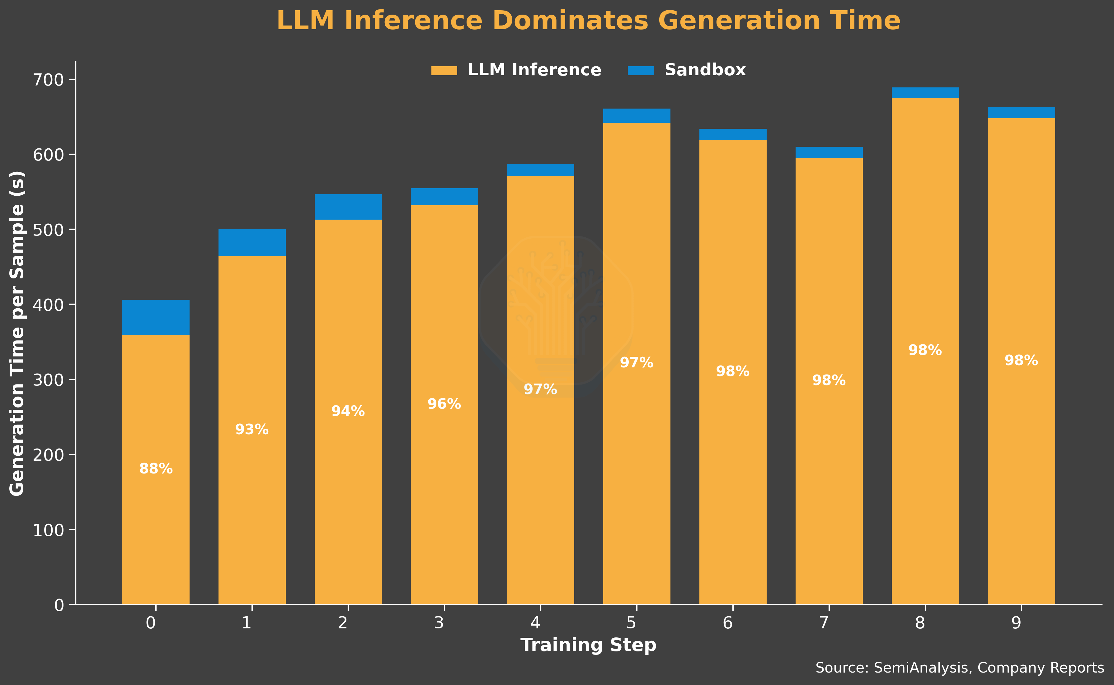
In this run, we see two factors set the system efficiency: model behavior drift and the curriculum being too easy for the model.
We observe both the average response length per turn and the number of tool calls (20 to 51) triple over the run. Together they push sequence lengths up and shift the workload toward a prefill-heavy profile. This supports our choice of disaggregated serving, which improves the worst-case time-to-first-token (TTFT) for prefill requests.
On the capability side, the curriculum is too easy for the model. On average, 55% of problems have a 100% solve rate, i.e., every rollout in the group passes. A rollout group where every rollout has the same reward produces zero advantage and contributes no training signal. As a result, average reward stays flat. The curriculum mismatch reduces the effective training samples and subsequently the effective generator production rate.
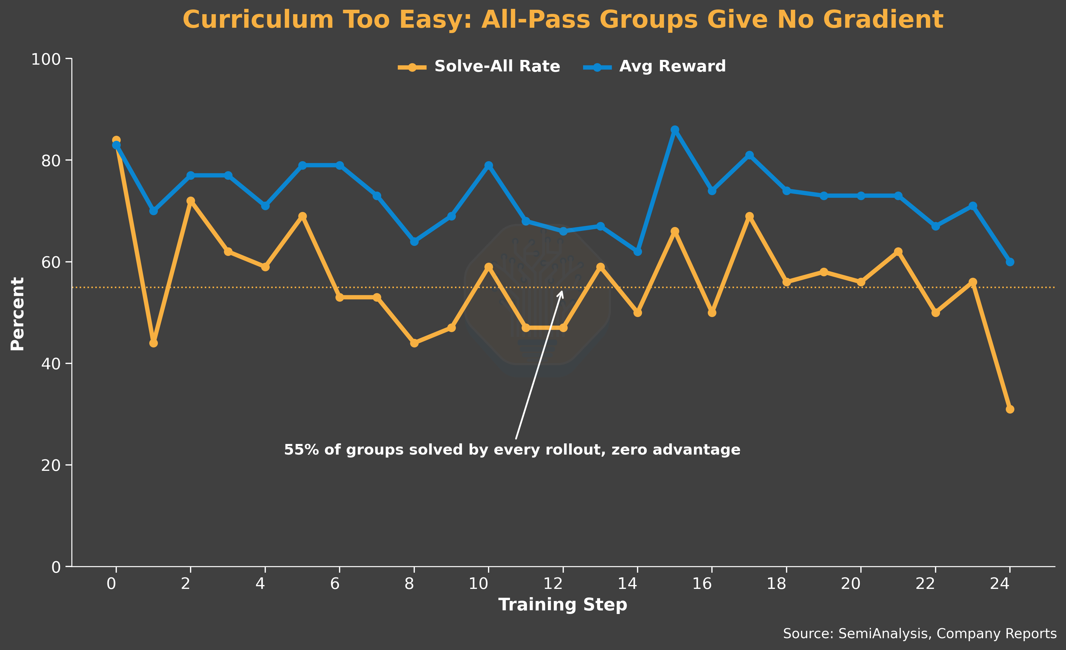
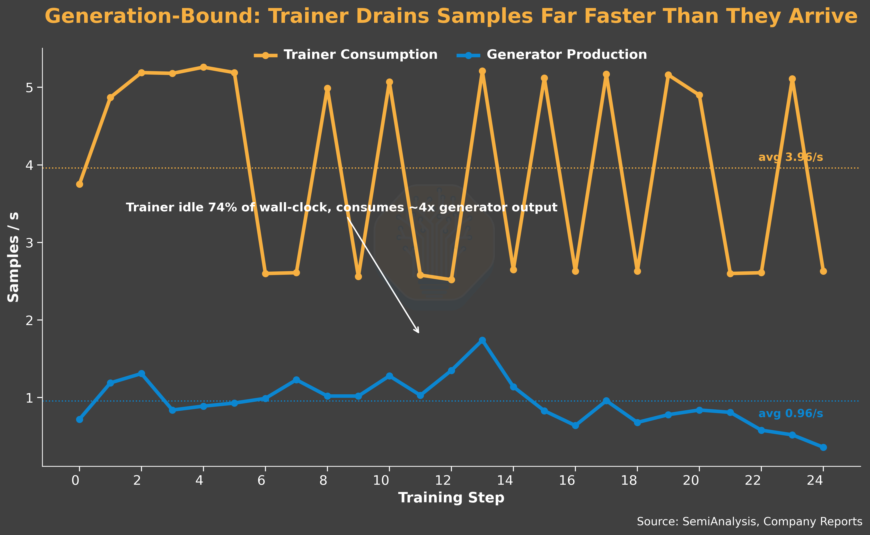
All the effects result in a heavily generation-bound system. The queue fills up fast, but a large portion is filtered out, so the output is low. LLM inference dominates end-to-end generation time and keeps growing as training progresses. The trainer spends 74% of the wall-clock time waiting, and its consumption rate is 5× the generator’s delivered production rate.
Sandbox Scaling Challenge
Setup
Model: Qwen3 235B A22B Instruct 2507, both FP16
Hardware: GB300
RL framework: verl + uni-agent rollout
RL environment: SWE-bench-style env, with Modal sandbox
Algorithm: GRPO
Max sequence length: 128K
Training Stages
1st Stage:
Trainer: 32 GPUs, TP16 / EP32, CPU offload
Generator: 24 GPUs, 6 replicas, TP4
Group size: 8
Number of concurrent rollouts: 96
2nd / 3rd Stage:
Trainer: 48 GPUs, TP4 / CP4 / PP3 / EP16, CPU offload
Generator: 24 GPUs, 6 replicas, TP4
Group size: 8
Number of concurrent rollouts: 256 (2nd) / 360 (3rd)
Analysis
The training dynamics were roughly in line with our other Qwen3 235B training runs. The run was generation-bound: trainer idled 30% to 60% of the time. Generation length grew aggressively: 3 to 8% of the samples hit max sequence length 128K, and for similar reasons, the tail latency blew up to 7500s for a noticeable straggler on step 9.
The unique part of this case is that we pushed the concurrent rollouts and encountered sandbox scaling issues. Scaling concurrent rollouts is critical to sample generation throughput. It enables higher batch size, more reward signal variance, and subsequently provides a better training signal. However, each rollout corresponds to at least one sandbox, and scaling rollout concurrency challenges the sandbox infrastructure reliability. In this case, we experimented with concurrent rollouts ranging from 96 to 960. At 960, once we pushed past our account's configured limits, we encountered sandbox initialization dead errors and straggler 1-hour sandbox spin up latency, and to mitigate that, we scaled down to 96, but then observed low rollout efficiency. This experiment shows how critical sandbox scaling is to RL training efficiency.
We thank Ao Shen and Kaichao You from vLLM / Inferact for helping conduct this experiment. The detailed writeup of errors and attempts is here, the WandB logs of the final stage training are here, and the code repo is here (verl, uni-agent).
Partial Rollout and Stateful Sandbox Design
Setup
Model: Qwen3-235B-A22B-Thinking-2507-FP8 (FP8 generation, BF16 training)
Trainer: 32x H200 GPUs, TP4 / CP4 / PP2 / EP8
Generator: 64x H200 GPUs, 8 replicas, TP8 / EP8
32K max sequence length, global batch size 64
Algorithm: GSPO, group size 8
RL framework: slime
Async setup: Fully asynchronous + partial rollout
RL env: SWE-Bench Verified and Lite, with OpenHands harness and Modal sandbox
Code repo: slime SWE Bench example
Analysis
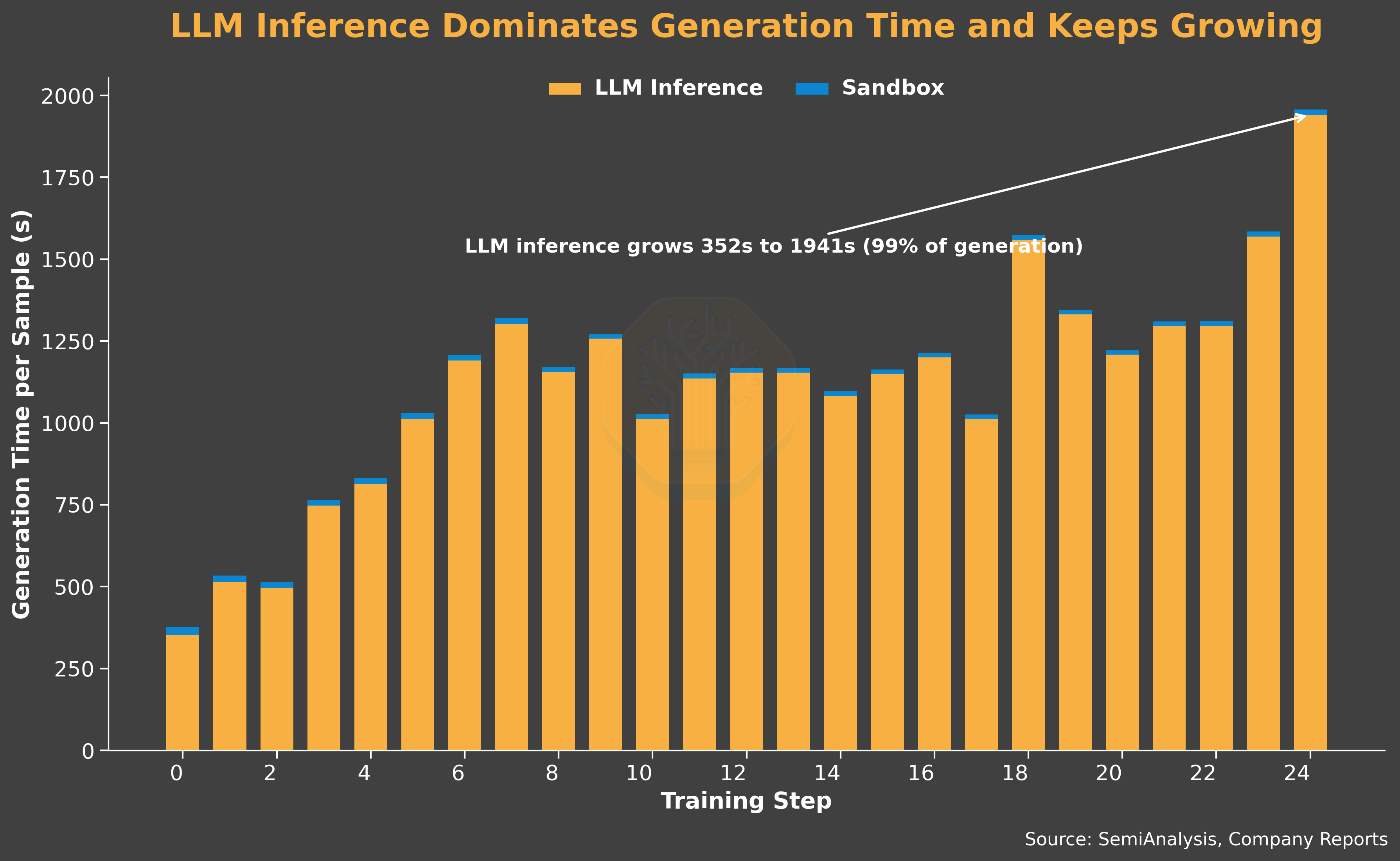
Overall, this experiment has system characteristics similar to other Qwen3 235B runs: generation-bound with 60% trainer wait ratio, long 12K response length per turn, a moderate average 12 tool calls per sequence, and a relatively low resolve rate.
We’d like to highlight slime’s partial rollout feature and how the sandbox design has to adapt to support it. Partial rollout allows the straggler rollouts to be saved into a buffer and restarted in a later batch. This mitigates the long tail latency of straggler rollouts, which improves system efficiency.
In slime, partial rollout marks straggler rollouts as aborted, saves them to a replay buffer, and puts them into the queue in future batches. This creates challenges for the sandbox:
Sandbox needs to persist across rollout batches, since SWE-Bench problems can be stateful: a partial rollout may be in the middle of editing files. This also means we need additional logic to track the sandbox ID and sample mapping
Sandbox needs to be lazily created: sample processing logic is coupled with sandbox creation, but there may be cases where the sample fails to emit tool calls, and creating a sandbox in that case would be wasteful
Sandbox robustness to failure: If sandbox fails during the time between a sample being aborted and being restarted, we need extra logic to ensure correctness. Since we didn’t figure out how to do failure resumption on Modal, we opted to mark the sample as failed
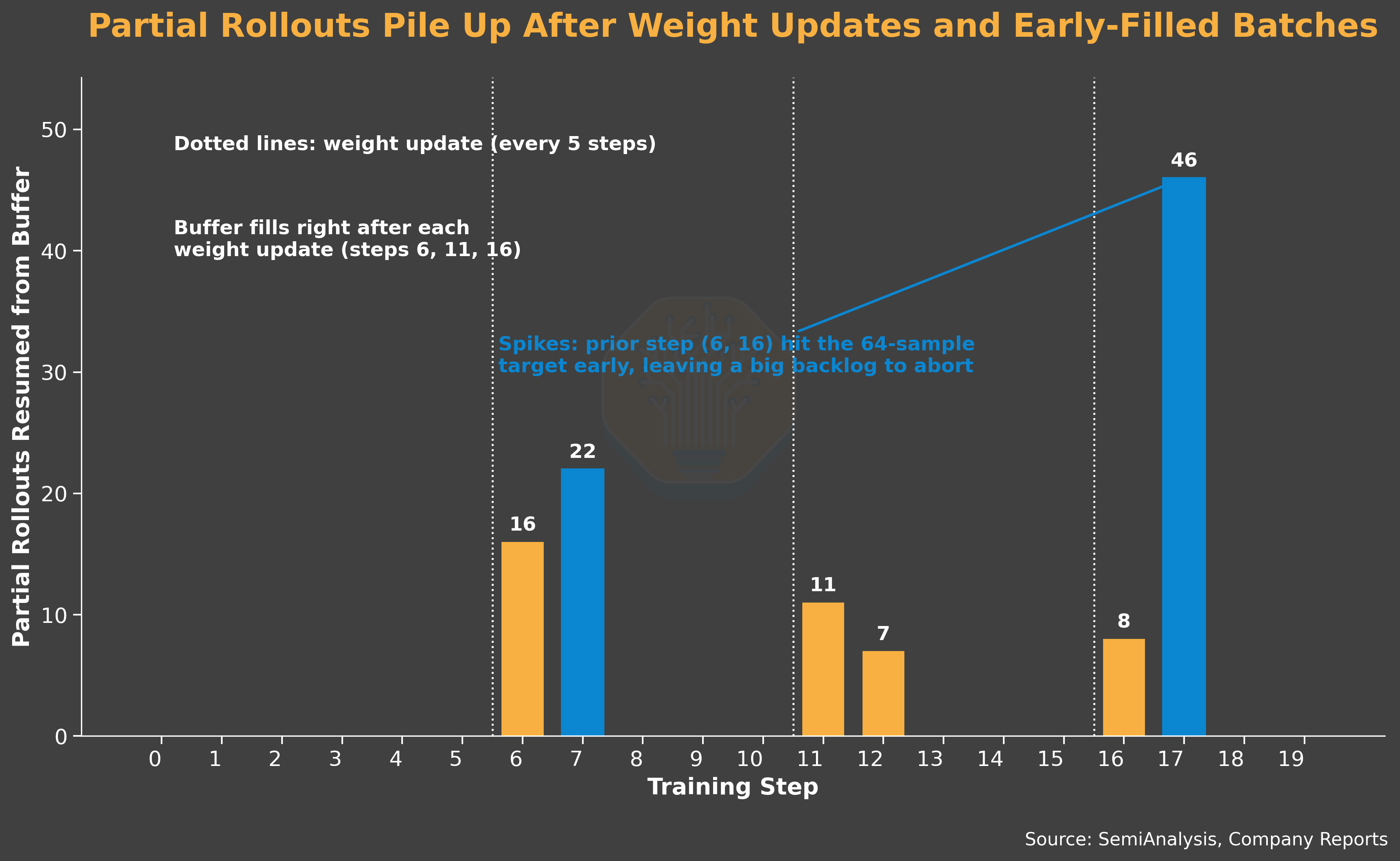
Slime triggers partial rollout abortion in two situations: when a target rollout batch is filled (64 samples in our case), and when the trainer pushes a weight update. This leads to an interesting dynamic of partial rollout count in the replay buffer. We see the number increase after steps 5, 10, and 15, since we update weights every 5 intervals. We also see the number spikes at step 7 and 17, and we believe it’s due to the previous step (step 6 and 16) completing as soon as it reaches the target rollout batch, leaving a big backlog.
Unlike PipelineRL, slime’s SGLang configuration evicts the KV cache for aborted rollouts. This means resumed rollouts are essentially large prefill requests, which is exactly the workload type that benefits the most from PD disaggregation.
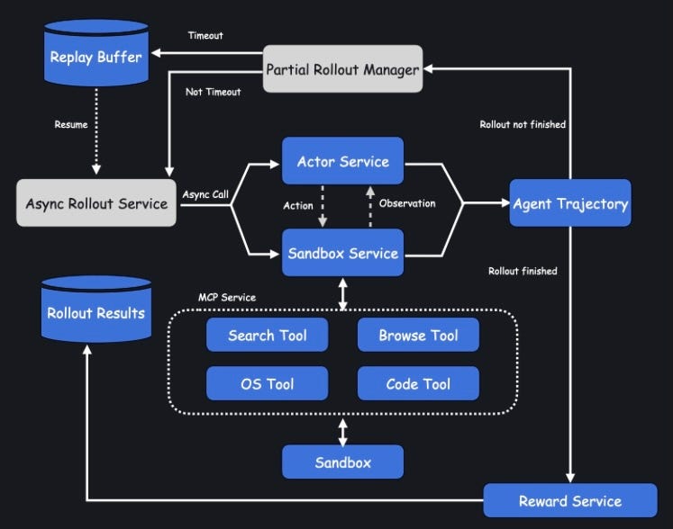
Partial rollout is where environment state-level staleness shows up. When an aborted rollout resumes in a later batch, the trainer has pushed new weights in between, so the resumed rollout faces not only the policy gap, but a state gap that’s specific to stateful environments. In our SWE-Bench case, the sandbox it wakes up in is not a fresh repo. The sandbox holds the half-applied edits, created files, and working-directory state that the old policy produced over its earlier turns. The newer policy now must continue from a situation it didn’t create and wouldn’t necessarily have created itself. This can corrupt the training signal: during training, the advantage gets attributed to a trajectory the current policy only partially owns. Seeing the high resume rollout count after weight updates, we suspect environment state-level staleness contributes to the run’s low resolve rate.
In summary, partial rollout rescues the stragglers to maintain the queue-filling throughput, but it comes at the cost of stateful-sandbox complexity and explicit environment state-level policy staleness.
Software User Experience
Prime RL
Prime RL has great user ergonomics. Users perform most commands with uv and configure setups in the .toml files. Prime RL also comes with agent skill files, allowing users to use AI agents more smoothly when working with the repo.
Regarding system design, we appreciate that Prime RL has an “orchestrator” actor to clarify who manages the trainer-generator dynamics. We love the hub of RL environments Environments Hub and look forward to it continuing to grow. Prime RL uses Torch Titan for training, vLLM for generation, and their in-house Prime Sandbox for hosting RL environments. Prime RL also supports PD disaggregation for the generator, which greatly boosts performance on agentic RL training. Overall, the codebase is lean and has most state-of-the-art techniques.
However, we also encountered some rough edges. Prime RL’s heavy reliance on uv assumes users have great familiarity with uv. We spent a lot of time compiling and re-installing flash attention 3 because we couldn’t figure out why uv uninstalled it. We encourage Prime Intellect to provide more resources to educate users on how uv works, in addition to the docs saying what uv commands not to execute.
Although Prime RL assumes it runs on a SLURM cluster, it assumes jobs run on bare metal instead of Pyxis. When we ran into CUDA library version mismatch for DeepGEMM libraries, running jobs in containers would solve the issue more easily.
We also had a lot of failed runs that turned out to be Prime Sandbox failures. We had a hard time parsing through Prime Sandbox’s error messages, which usually happens late into the run.
Errors include dangling sandboxes using up sandbox quota, out-of-resource errors, out-of-credit issues, many of which can be detected before launching a run. Prime Sandbox is still in beta, so we expect it to improve in the future.
We thank Prime Intellect for supporting the effort, including software and hardware resources. Prime Intellect provided training recipes based on this PR (Commit hash here).
slime
slime is known for its clean and minimal abstractions, and we believe it lives up to the hype. We particularly like slime’s hook abstractions. They allow us to write customized functions for rollout processing, reward functions, and metric logging utilities. The function signature and contracts are clear, and it’s a breeze to integrate and add new features during development.
We also want to highlight how friendly and helpful slime’s developer team is. Zilin, slime’s core maintainer, has offered guidance on configuration tuning and answered slime design questions.
Our main gripe is slime’s focus on co-located mode, and as a result sparse documentation of asynchronous modes. We figured the difference between async and fully async and the mechanisms of partial rollout mostly through trial and error. We hope slime can provide better documentation on those topics.
Modal
Modal has great API documentation: We referenced Modal’s Sandbox API extensively when implementing the sandbox integration in slime, and the documentation is clear and helpful. Modal services have also been relatively robust throughout our experiments. Under small scale, Modal has been reliable, and creating / terminating sandboxes is easy and responsive. The Modal team has also been very friendly and helpful. Modal offered support early on in our effort with API credits, and Modal’s slime integration team Peyton and Nan offered great advice and feedback on our experiment results.
The main challenges for Modal arose when we ran many concurrent sandboxes. As we reported above, we saw dead initialization errors and long-tail sandbox start-up latencies. We suspect this was our own misuse of the API rather than a hard limit in Modal, but we couldn’t pinpoint the root cause on our end during training. We later reached out to Modal and collaborated on identifying the issue. It turned out to be the resource limit on our account, and we were able to verify the stability of high sandbox concurrency after Modal raised our limits (Reproduction code here). We appreciate the responsiveness of Modal’s developer team, and we hope Modal can offer more sandbox observability tools and more documentation on how to scale sandboxes in the future.
History of Open-Source RL Frameworks
The release of DeepSeek R1 sparked the open-source community effort to reproduce the algorithm and infrastructure. One of the early efforts is OpenRLHF, a large-scale RL training framework that implemented PPO, REINFORCE++, and then GRPO. OpenRLHF profoundly influenced the subsequent RL framework developments. Numerous OpenRLHF maintainers later developed popular RL frameworks, including slime and verl. These frameworks created vibrant Chinese communities of RL training, which we believe positively contributed to recent advances of Chinese models. These open-source frameworks also enabled academic researchers to develop new algorithms and techniques, bringing RL research within reach of academia.
We thank Kaichao, who led vLLM’s early-stage RL integration in OpenRLHF, verl, etc., for sharing this history. We hope this shows that sincere collaboration and sharing, rather than hostile competitions and information hiding, propels science forward.
Conclusion
RL training system efficiency is a matter of queue health. Oversampling, early pruning, and partial rollout controls what enters the queue, adaptive sampling and policy staleness controls what leaves the queue, and in-flight weight updates allow trainer and generator to operate at different rates.
RL training is as much of an infrastructure problem as an algorithm one. In this post, we focused on systems, explaining how system and algorithm designs are intertwined, and grounding them with real-world experiments. We hope this ignites interest in RL infrastructure and bridges RL algorithm researchers with system engineers.
We plan to continue exploring the systems and infrastructure of RL training in our future articles. We will explore in depth techniques such as PD disaggregation and speculative decoding, and system challenges of large-scale RL training such as training Nemotron 3 Ultra. We are also looking into benchmarking sandbox infrastructure and analyzing model rollout traces.
If you’re interested in working on these topics, we’re hiring! Please contact us at letsgo@semianalysis.com . Attach your resume and ask us questions about this article.
For our last section, we present a TCO analysis of RL training, and we compare it to RL training platforms Tinker from Thinking Machines Lab. We quantify how much more cost efficient Tinker is, and we hypothesize the reasons behind it.