

Vera Rubin NVL72 is the second generation of Nvidia’s rack-scale Oberon architecture, and its gains on inference come from extreme co-design. Early results from engineering samples are encouraging. Vera Rubin NVL72 running DeepSeek R1 delivers 5.4x performance per MW and 5x performance per dollar over GB200 NVL72 today, and the gap is even wider against GB200 NVL72 during its early bringup in 2025. Vera Rubin is still in the early bringup stage now, so we expect the gap to continue widen. Rubin's inference performance will keep improving as software matures, the same pattern we demonstrated for Blackwell in our InferenceX benchmarks, and Rubin still has a long runway ahead.
Nvidia has also recently made available their first public release of the Rubin (SM_107) software stack with CUDA13.4 and has upstreamed Rubin PRs to PyTorch, vLLM and OpenAI Triton Compiler. Blackwell was not able to reuse Hopper WGMMA kernels, Rubin is able to reuse Blackwell's kernels, which makes the software bring up process much smoother. For speed of light (SOL) performance, engineers will still need to tune and rewrite kernels but for those that are focused on time to market, Blackwell kernels can be reused. We will also explain Rubin’s new 3 bit programmable LUT tensor core.
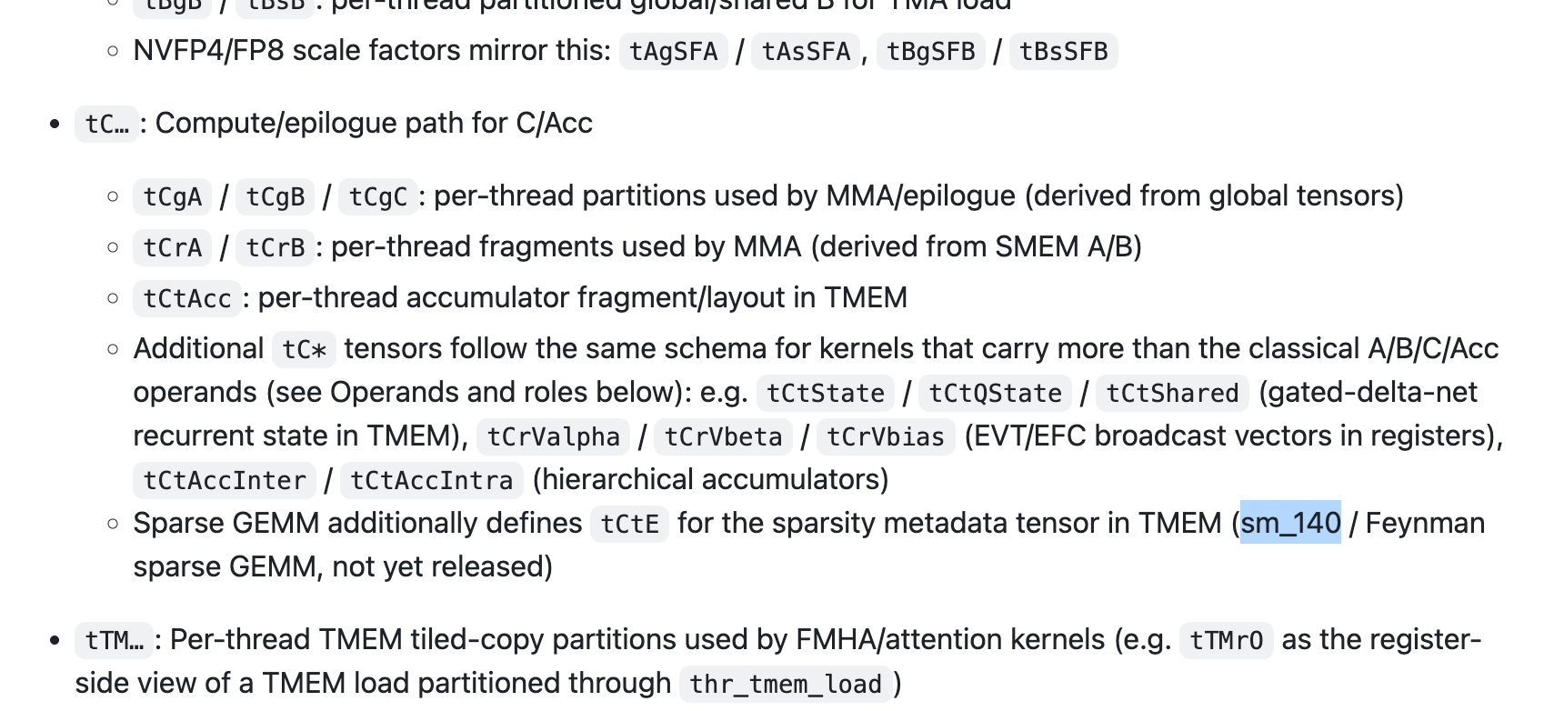
NVIDIA has also released on GitHub that Feynman is SM_140. Unlike Blackwell to Rubin, Rubin to Feynman will be an much more complex transition on the kernel front.

The early metrics gathered on VR NVL72 come from CoreWeave. We have not independently verified them. Nvidia has committed to submitting verifiable numbers to InferenceX by Q3 CY2026. Google should submit TPUv7 results in the next couple of months, and AMD has committed to MI455X UALoE72. Once those land, the ecosystem gets an objective comparison across systems.
In this article we break down Nvidia's Rubin claims against several baselines, showing where Rubin clearly leads Blackwell and where the lead is thinner. We will also analyze Rubin’s performance per total cost of ownership using our already existing estimates for Rubin’s total cost of ownership (TCO). The TCO for Rubin and many other systems is sourced from our AI TCO model, which tracks the total cost of ownership of different AI chips, factoring in capex, opex and different other expenses. We also consider performance per watt using our All-in Utility Provisioned Power Estimates from our Datacenter Model.
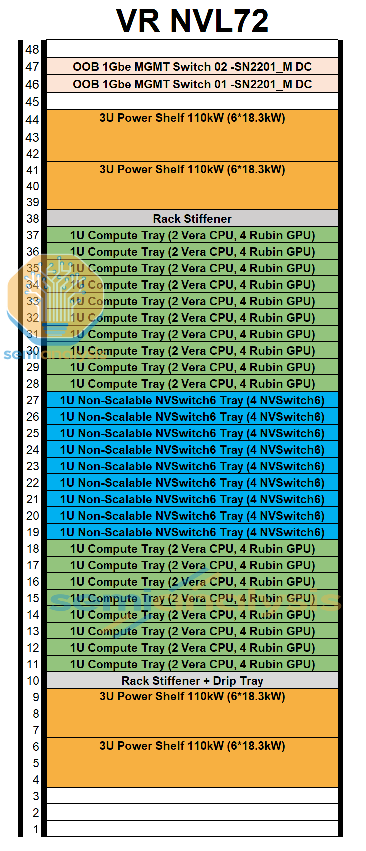
Finally, we will present a component by component build up of the Bill of Materials (BoM) for the VR NVL72. This is available in our upcoming SemiAnalysis Bill of Materials (BoM) Model.
Another area where Rubin Oberon NVL72 will fare better than Blackwell Oberon NVL72 is in a much faster production ramp period. This is thanks to Rubin’s simpler cableless compute tray design and learnings from Nvidia’s experience with deploying a rack-scale copper backplane, having invested much effort into ironing out issues with Blackwell’s copper backplane. Our Accelerator Model tracks quarter by quarter shipments of Rubin at both the package level and the rack level.
A Brief Breakdown of Rubin Chip-Level Microarchitecture Features
Going through a complete breakdown of Rubin microarchitecture will have to wait until we obtain ssh access to Rubin systems, allowing us to run benchmarks similar to those we carried out when first analyzing Blackwell. However, there are still a few interesting points we can still make.
We expect that Rubin bringup will be much more seamless compared to the transition from Hopper to Blackwell, where engineers expended much effort just to port kernels to Blackwell. This simplicity comes from the fact that Rubin is able to run Blackwell SM100-family kernels across all the important kernel libraries in DeepGEMM, FlashMLA, CUTLASS, among others. Moving from Hopper to Blackwell meant rewriting kernels from scratch. Hopper’s kernels don’t run on Blackwell at all.
Reusing Blackwell SM100 kernels means a clear time to market advantage, but for speed of light (SOL) performance, engineers will still need to tune and rewrite kernels specifically for the Rubin architecture, though kernel reuse buys them time to focus much more on this kernel tuning.
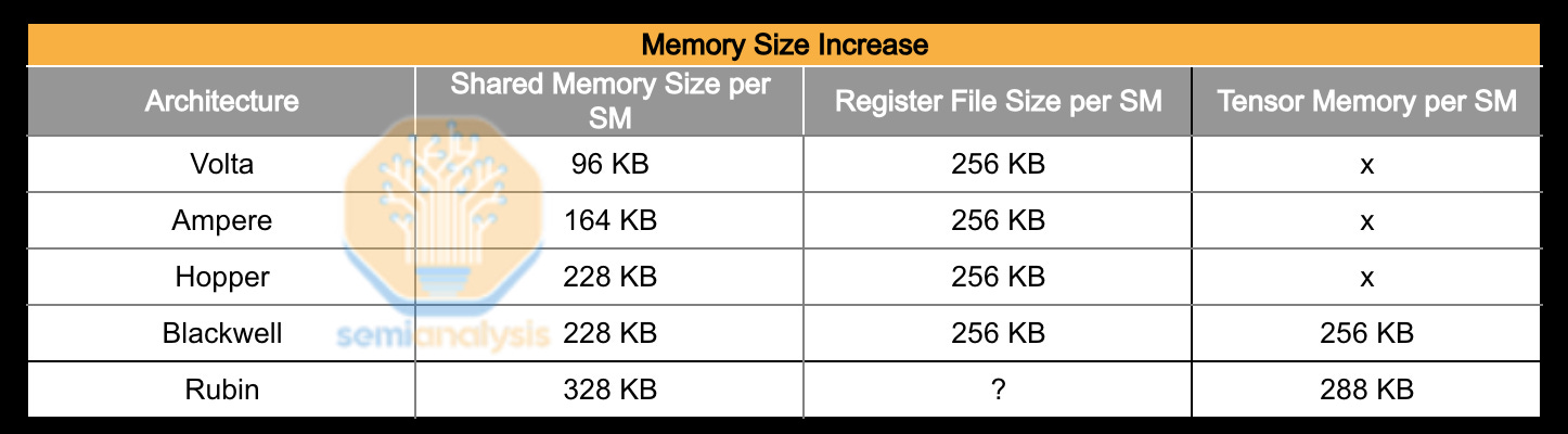
Turning to architectural details, Rubin’s SMEM increased to 328 KiB compared to Blackwell’s 228 KiB. While the default SMEM capacity is 228 KiB, Rubin comes with an oversized shared memory mode that allows increase to 328 KiB. Furthermore, TMEM has been increased to 256 KiB up from 228 KiB in Blackwell as the number of columns increased from 512 to 576. The additional columns will allow stashing block scale factors, while keeping the TMEM region for accumulators disjointed from it. This greatly simplifies block-scaled kernel logic: it saves the kernel writers from carefully pipelining and overlapping MMA matrix and block scaling factor loads.
Rubin's TMA now supports inline descriptor updates. There are tons of use cases for this. For example, in an MoE layer, each expert is a separate weight matrix at its own address in HBM, so the TMA descriptor has to point somewhere new on every expert switch. On Blackwell, that meant rewriting the descriptor in memory and synchronizing before the next load. Now, with Rubin, the per-expert offset is passed inline to the TMA instruction so that one descriptor covers all experts, with no in-memory rewrite between them. This removes overhead during token dispatch and improves decode speed at low batch sizes.
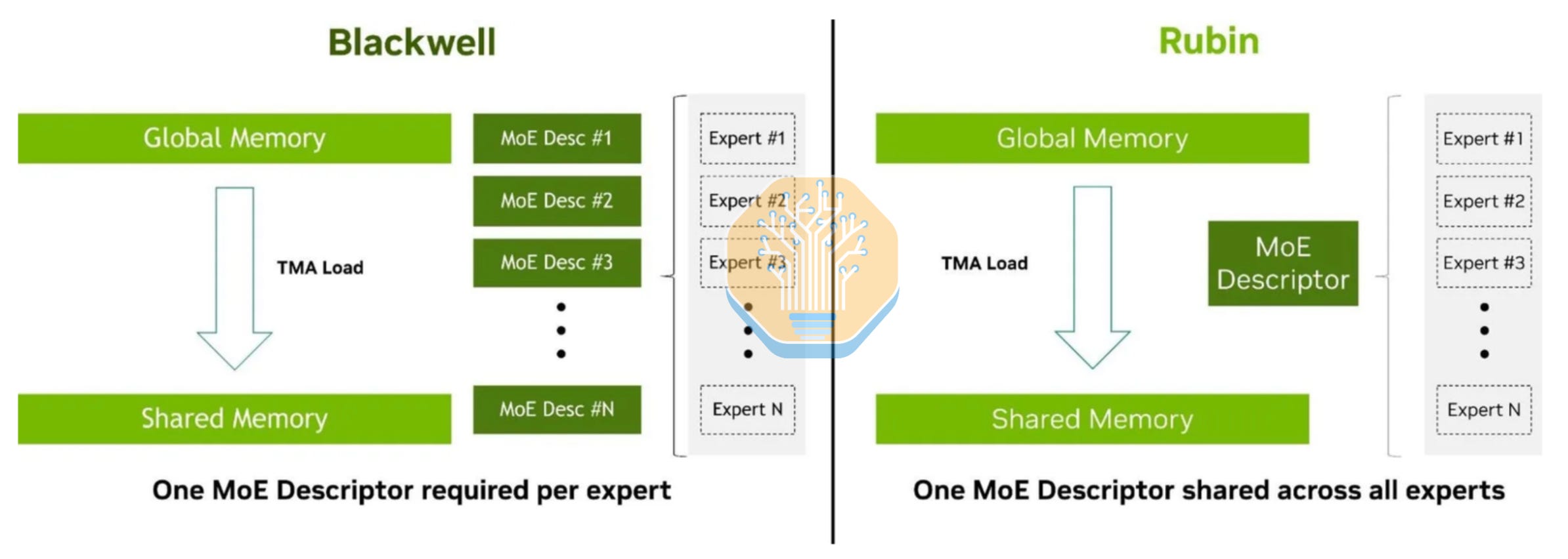
Inline TMA descriptor update corresponds to the ISA feature .override qualifiers. TMA instructions require a tensorMap object that specifies layout and format metadata. By using the .override qualifier, bulk asynchronous copy instructions can reuse the tensorMap object as a template, but replacing certain metadata fields, such as strides. In the case of MoE, expert weights have identical shapes, data types, and properties. By overriding the global address, kernel writers can avoid duplicating or replacing tensorMap objects when loading different experts.
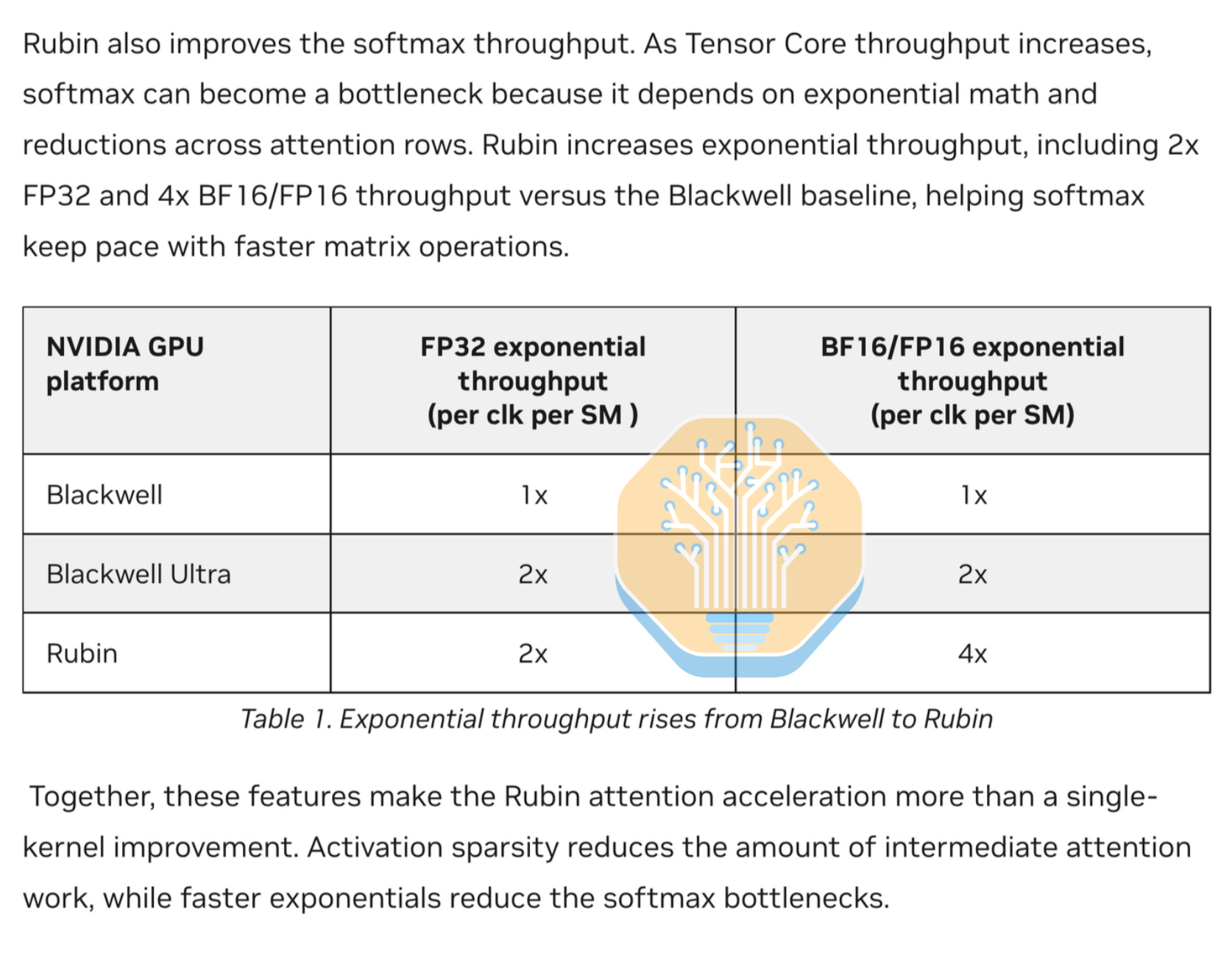
Rubin doubles BF16/FP16 exponential throughput per clock per SM again, which helps overlap Tensor Core work with softmax during attention. FP32 throughput is unchanged from Blackwell Ultra.
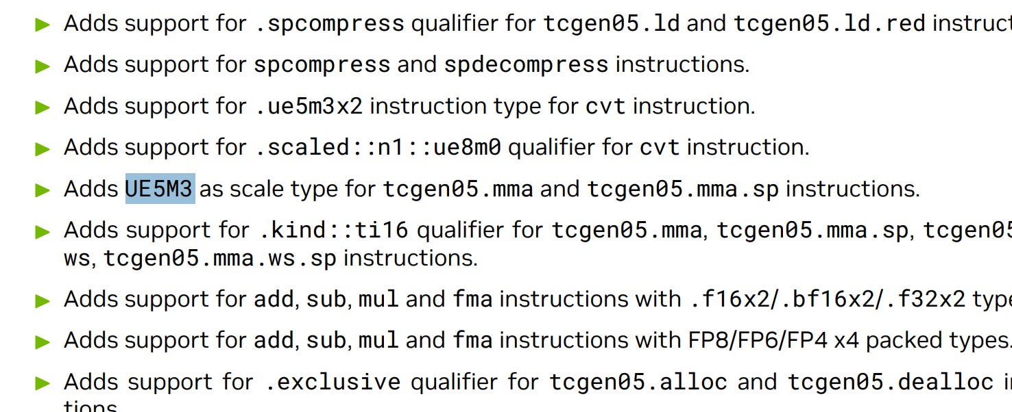
Compared to Blackwell NVFP4/MXFP4 Tensor Cores which could only accept UE4M3/UE8M0 block scale factor format, On Rubin Tensor cores, it will now be able to accept UE5M3 8 bit block scale factor too. This additional block scale format will allow for more flexibility and less quantization error is certain cases due to its wider range.
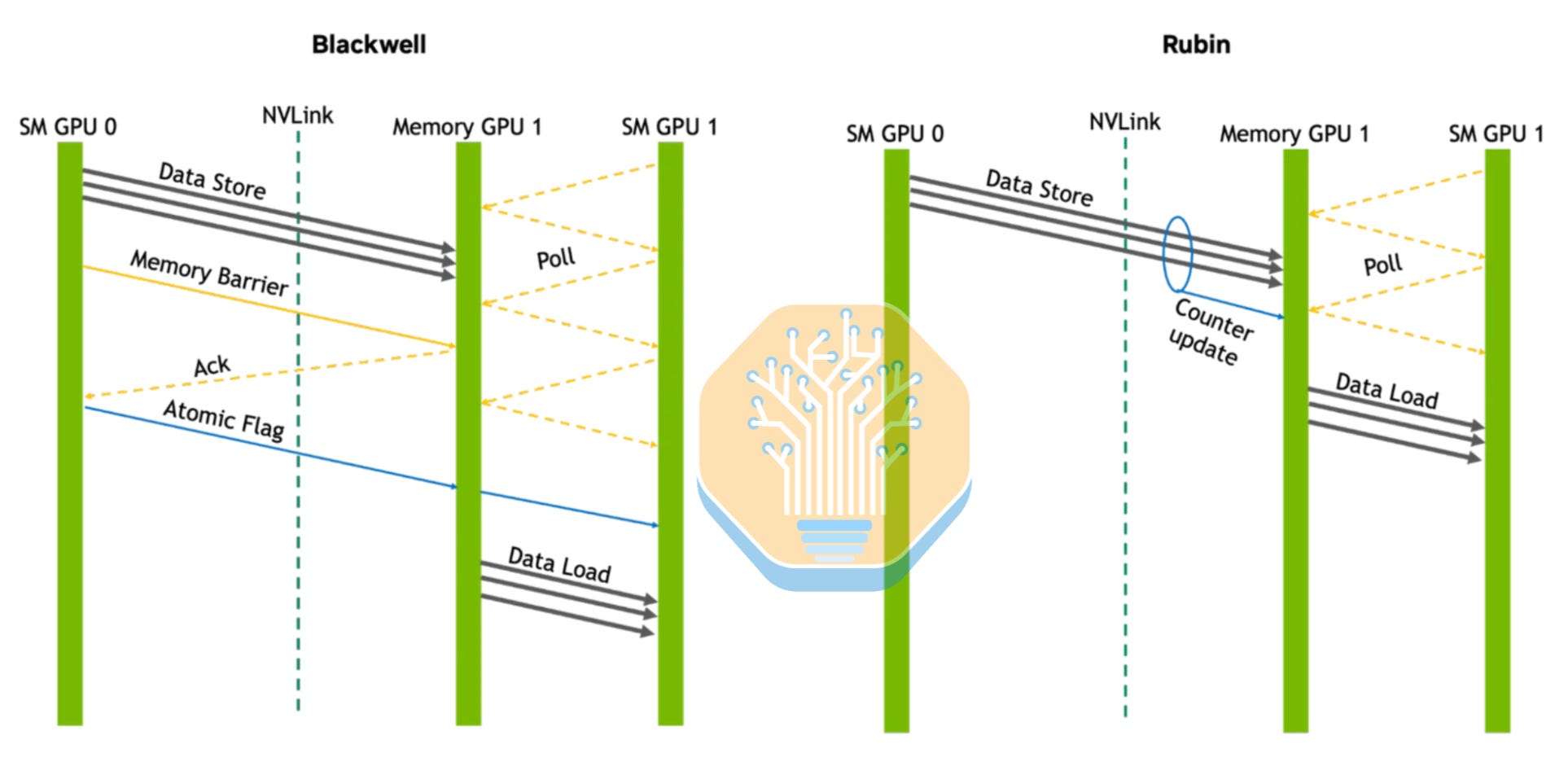
It is also important to note that latency has improved for SM-driven NVLink communications through the use of counted writes, which reduces the number of back and forth messages required to send data between GPUs over the copper backplane. This is a huge deal because Blackwell NVLink latency is multiple times higher than that of TPU and Trainium.
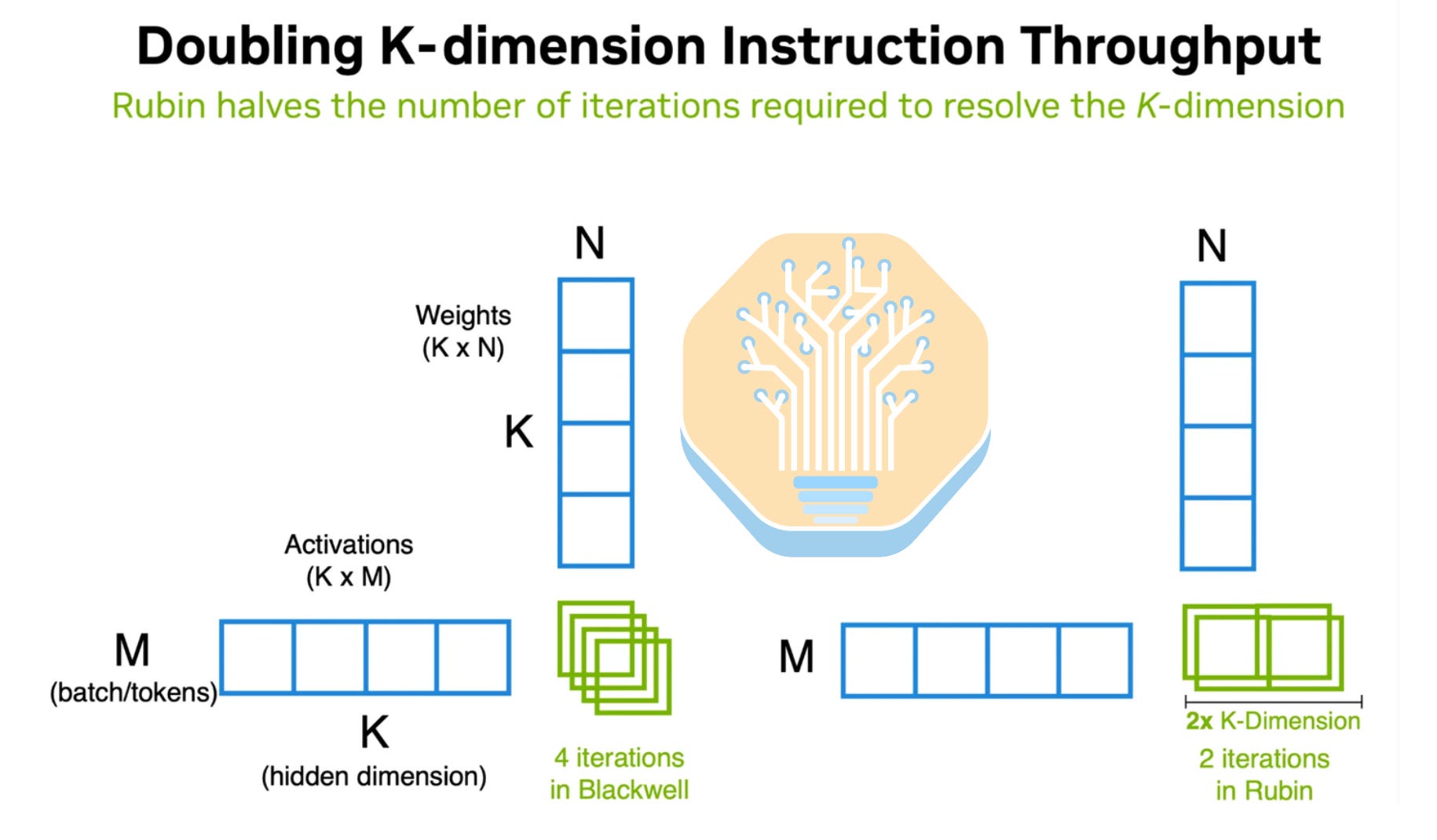
Rubin’s Tensor core delivers twice the throughput for FP8 and FP4 as compared to Blackwell. A key change driving this is doubling the k dimension as this means in theory, a GEMM takes half the number of clock cycles to execute. Additionally, the awkward K=96/3xFP4 instructions from Blackwell Ultra are still present, but alongside a new K=128 variant.
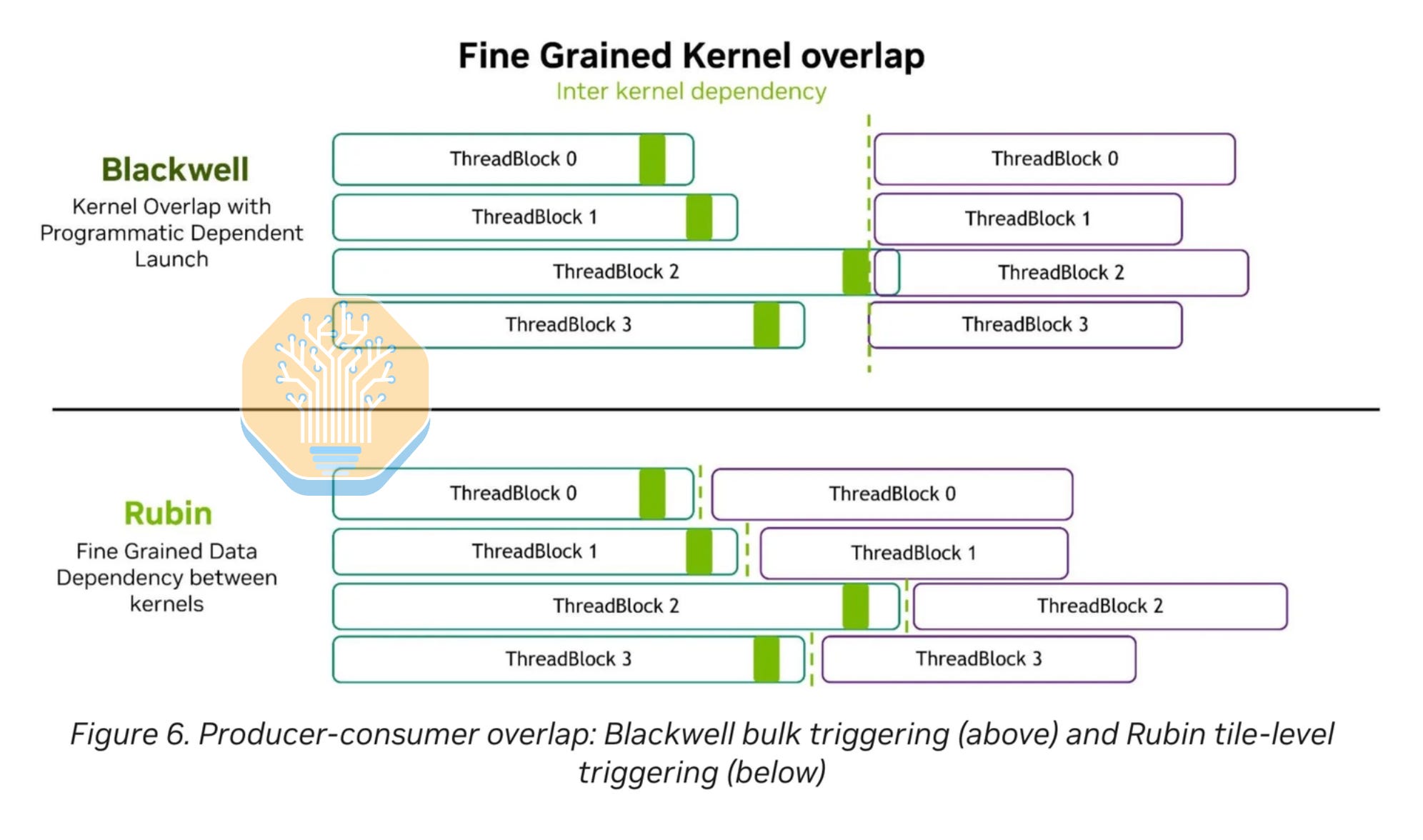
In Blackwell, PDL allowed for overlap at the grid level, where the dependent grid needs to wait for all threadblocks in the previous kernel to complete before starting. This allowed for some overlap and hiding of the ramp-down and ramp-up time between kernels, but didn’t come close to the extremely fine-grained overlap that trendy megakernel authors look to achieve. In Rubin, finer-grained overlap is enabled, where the dependent kernel can synchronize with the previous kernel at the threadblock level instead.
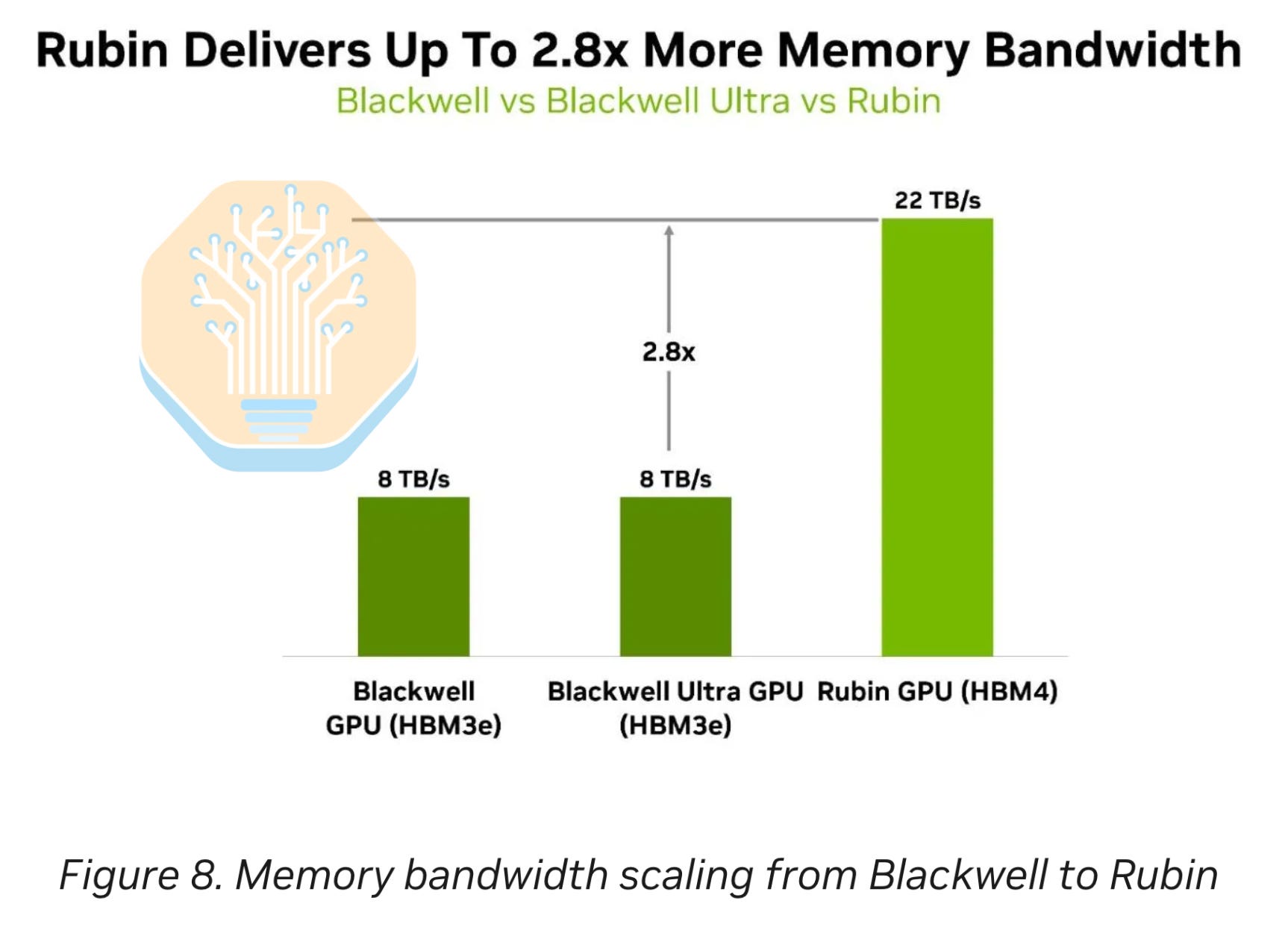
Rubin has 2.8x higher global memory bandwidth than Blackwell Ultra through the use of 3D-stacked HBM4 memory. It is unlikely Rubin delivers any improvement versus Blackwell in memory system latency. Our Accelerator & HBM Model has an complete breakdown of the memory volumes estimates & vendor used in Rubin.
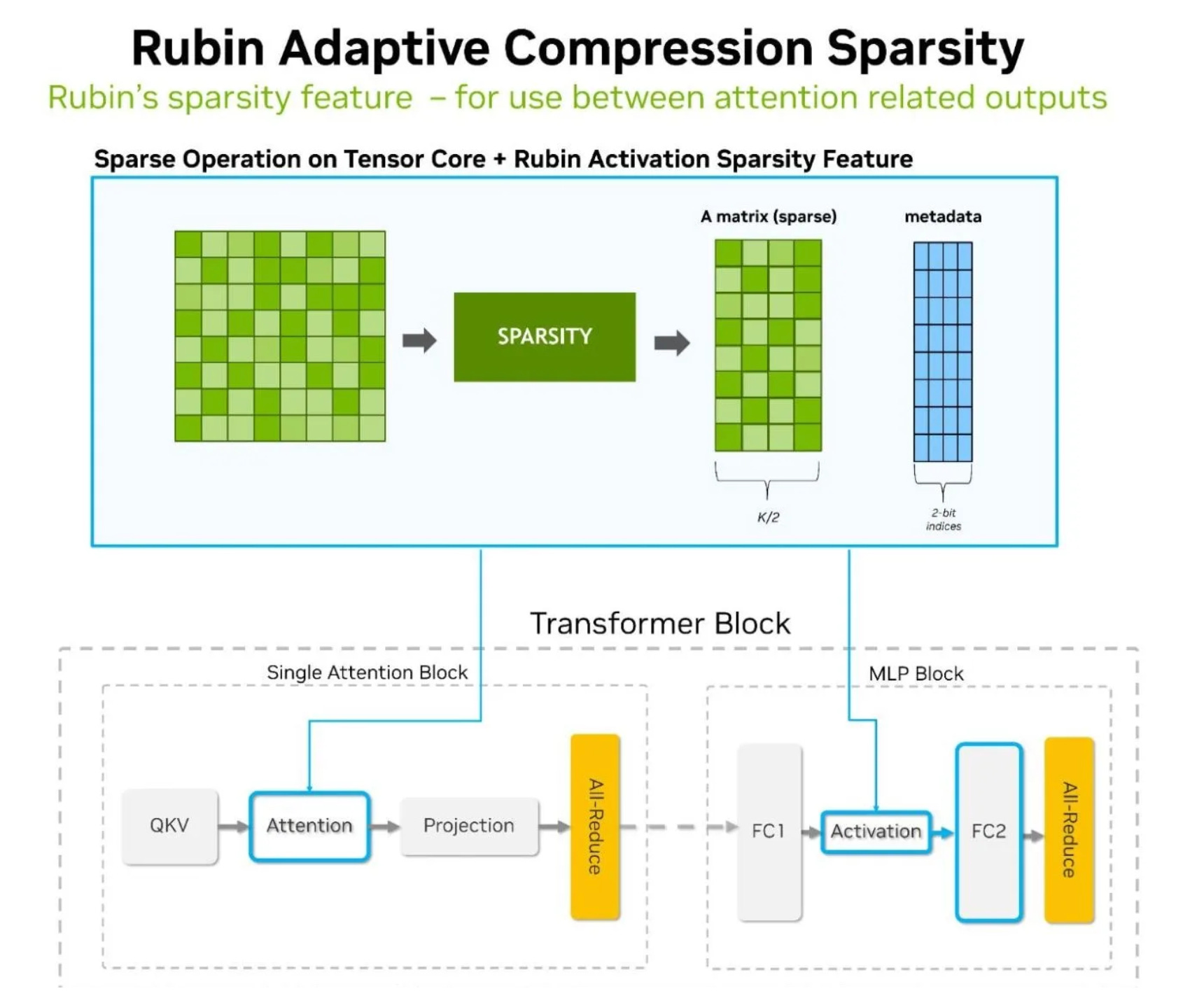
Rubin adds 2:4 sparsity support for activations. In every group of four values, two are kept and two are zeroed. The pattern is regular, so the Tensor Core knows where the survivors are, skips the rest, and runs the MMA at twice the rate. A small metadata field tracks which slots were kept.
Nvidia shipped 2:4 on weights back in Ampere and nobody used it, because it meant pruning the model and retraining. Rubin applies it to activations at runtime, so no retraining is needed. In attention, QK^T runs dense, then the scores get compressed on the way out of Tensor Memory. Softmax processes only the survivors, and the following GEMM against V runs sparse. The output stays dense, so nothing else in the model changes. It works on MLP activations too.
Nvidia has published no accuracy data, and throwing out half the attention scores before softmax is not obviously free. CoreWeave’s DeepSeek R1 results do not appear to use it either, which makes it another Rubin feature with silicon today and no tuned kernels behind it yet.
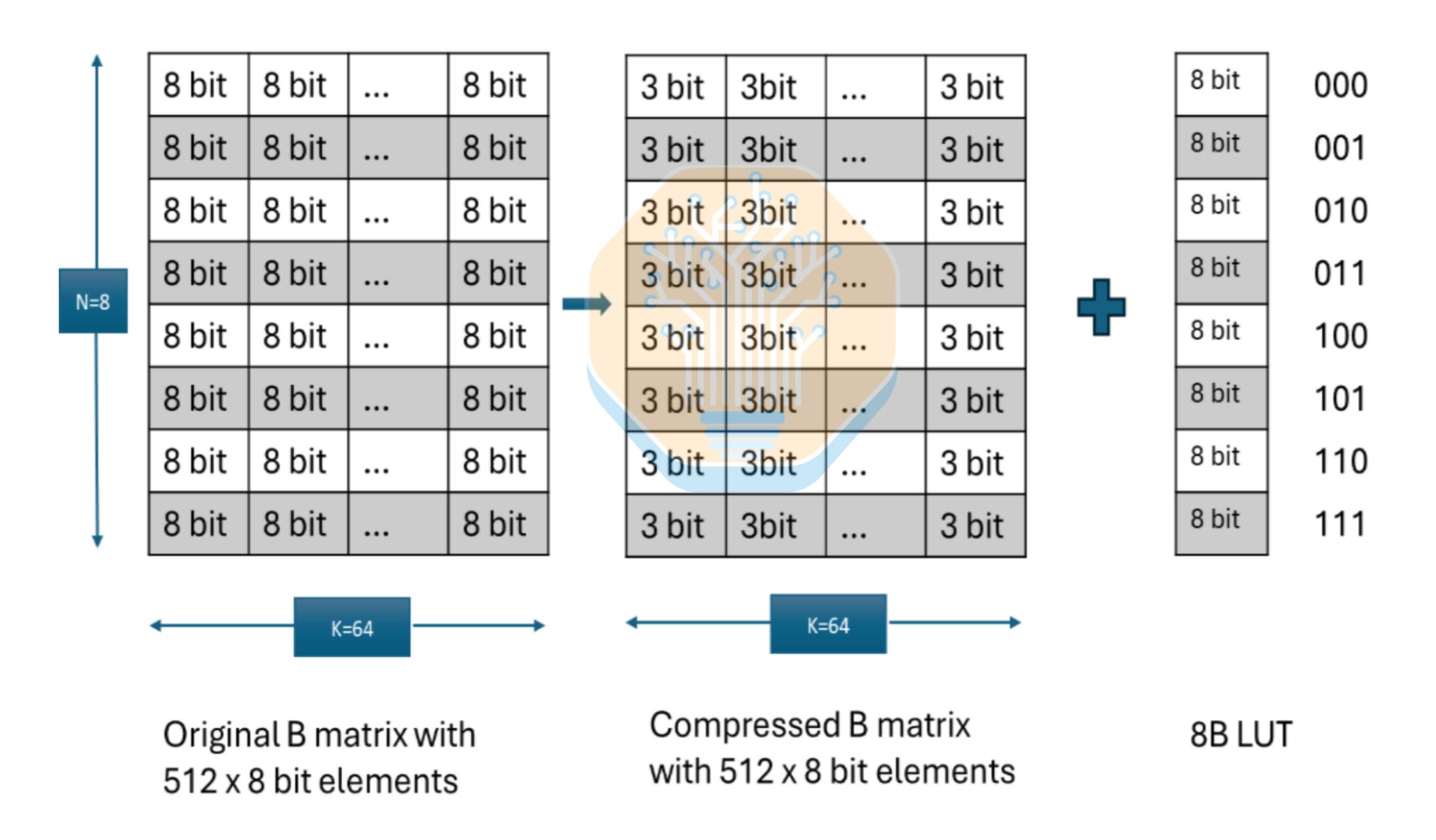
Lookup Table Weight Decompression in Rubin SM107 Tensor Core
Rubin adds LUT B, a Tensor Core MMA mode that decompresses the weight operand from a lookup table. In this mode, the B operand is a compressed matrix of indices. In a standard inference GEMM, the B operand holds the weights. The weight values live in a lookup table in Tensor Memory. The Tensor Core reads each index and reconstructs the weight value inside the MMA. There is no separate dequantization pass. After lookup, the multiply runs at FP8.
In LUT B, every weight position stores a 3-bit index rather than a complete numerical value. The index selects one of eight E4M3 values in the lookup table shared by that weight’s 8×64 block. For example, if the stored index is 5, the Tensor Core uses entry 5 from that block’s lookup table as the weight. The lookup happens inside the MMA, so the kernel never has to construct a separate decompressed weight matrix.
The lookup table (LUT) does not have to follow the spacing of a conventional uniform or floating-point grid. A quantization algorithm can therefore place more values around dense clusters of weights, use uneven spacing for long tails, or choose an asymmetric codebook when positive and negative weights have different distributions.
This flexibility creates the possibility of better accuracy per stored bit. Rubin LUT B has fewer individual codes than FP4, but it can place those codes where a particular weight group needs them rather than accepting the fixed ratios of E2M1. It is not automatically more accurate than MXFP4 or NVFP4, however. One codebook is shared across 512 weights, whereas NVFP4 adapts its scale over much smaller groups of 16. The result will depend on the codebook-fitting algorithm, calibration data, quantization-aware training and whether sensitive layers remain at higher precision.
Each index is 3 bits while the lookup table has 8 entries. Each entry is one byte, an E4M3 8-bit float in the reference kernel. This results in 3.125 bits per weight: 3 bits for the index, plus 64 bits of codebook spread across 512 weights. The codebook sits in HBM with the indices, so 3.125 bits per weight is the full stored footprint.
The instruction loads the compressed weights into the collector buffer. The Tensor Core can hold them there and reuse them across a run of activation tiles. This is a weight stationary pattern. The mode also has limits as it does not support transpose of the B matrix.
The block-scaled formats, NVFP4 and MXFP, also decompress inside the MMA. But they apply one uniform scale per block, not a codebook. Software methods like AWQ reach low bit counts by running a separate dequantization step before the matmul, Rubin is the first NVIDIA Tensor Core input format that reconstructs a non-uniform codebook inside the MMA.
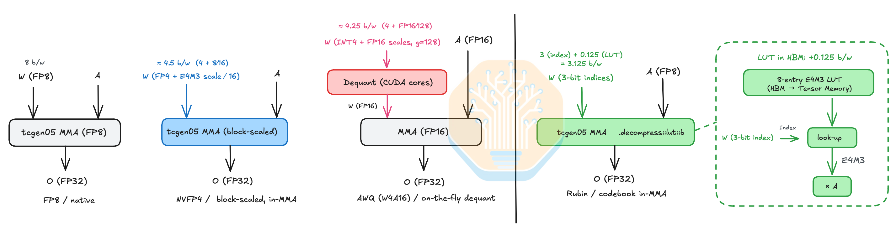
A lower bit rate cuts the HBM capacity that the weights need. It also cuts the bytes that the GPU reads for each weight. At low batch size, weight bandwidth limits the decode step. Fewer bytes per weight then raise decode throughput. A non-uniform codebook also holds accuracy better than uniform rounding at the same bit count. This feature should also have an impact on power efficiency, as fewer bits will need to move through the memory system for each flop.
Using Kimi K3 2.8T as an example, at about 4.5 bits per weight, MXFP4 stores 2.8e12 x 4.25 / 8 = about 1,4875 GB, where GB = 1e9 bytes. At 3.125 bits per weight, the Rubin lookup-table format stores 2.8e12 x 3.125 / 8 = about 1,094 GB (about 1.09 TB). The difference is about 393.5 GB. These figures cover the raw weight payload only, and exclude the KV cache, activations, and any parallelism replication. At 288 GB of HBM4 per Rubin package, the weights alone need about 6 packages in NVFP4 and about 4 packages in the new Rubin format.
Feynman Architecture Sneak Peek
From Blackwell (SM100)/Blackwell Ultra to Rubin (SM107), the jump is relatively small in terms of the microarchitecture, so Rubin can be thought of as a Blackwell kicker architecture. In comparison, Feynman (sm_140) is a completely new architecture family. This will require rewriting lots of kernels from Rubin to Feynman, which is similar to what happened from Hopper WGMMA to Blackwell tcgen05. Our Accelerator & HBM Model provides a full breakdown of Feynman quarter by quarter volume estimates.
Feynman’s 3D stacking will be similar to what AMD has been doing with 3D stacking since their MI300X with CDNA3.
One of the new features of the Feynman architecture is that it will contain sparsity aware data movement ops. These can be used in sparse GEMMs to improve performance by avoiding pointless loads, stores and FMAs.
Nuances of CoreWeave VR NVL72 Results
Yesterday, CoreWeave published their benchmarked Vera Rubin NVL72 Inference results expressed in units of performance (tokens/sec) per power used (MW). We will break down the nuances of their data and compare their results against Blackwell’s performance using our own InferenceX July 2026 results as a baseline.
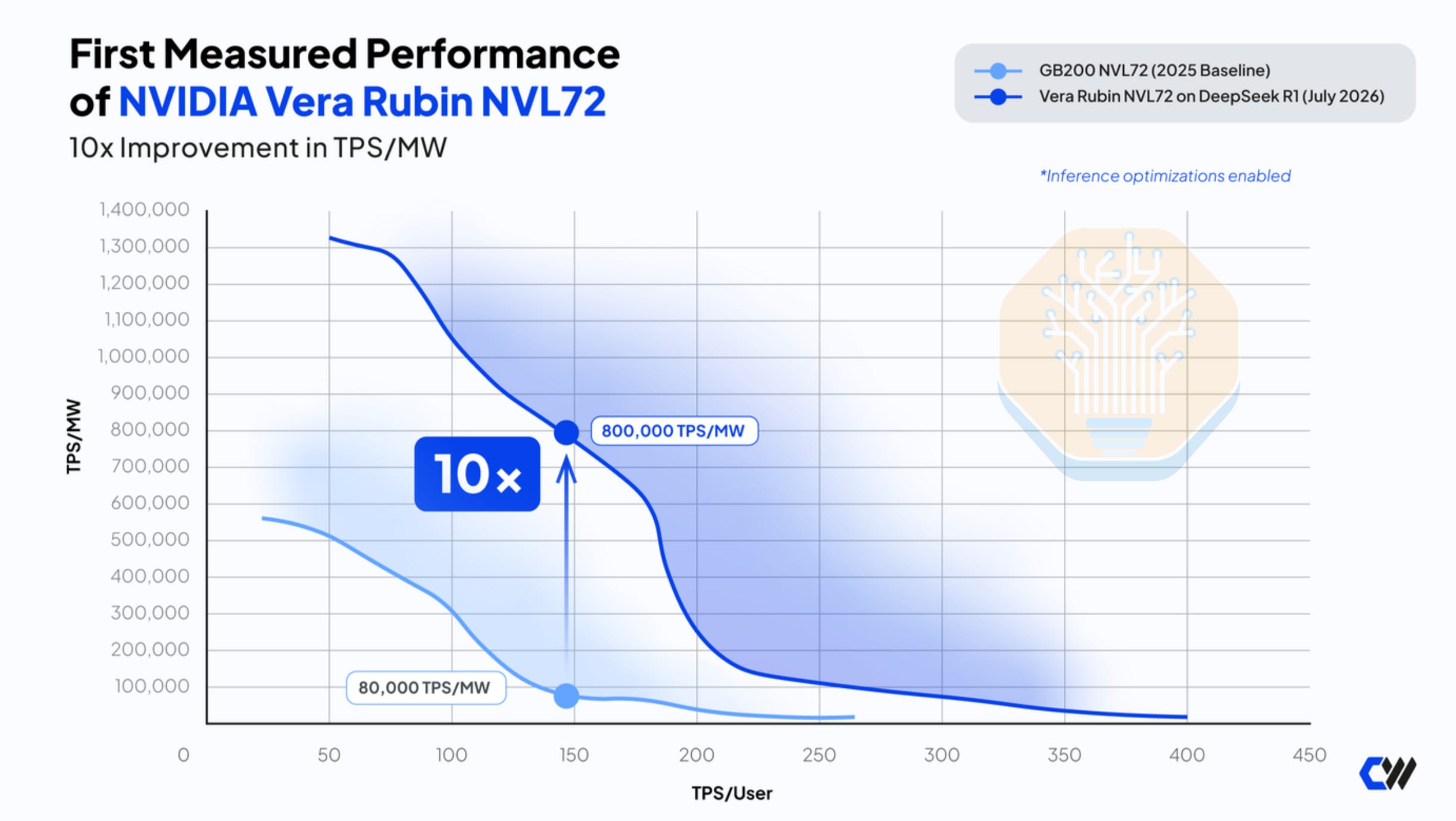
The first notable claim on the CoreWeave-Nvidia chart is that VR NVL72 achieves 10x better token throughput per megawatt than GB200 NVL72 at the iso-interactivity of ~150 tok/s/user. This is about 50% faster than today’s “fast mode” on frontier models.
Three things about their chart. The benchmark is single-turn, 8k in and 1k out. The y-axis is output token throughput per megawatt, not total throughput. And their power number covers both prefill and decode GPUs, even though only output tokens are counted. InferenceX measures output throughput against decode GPU watts only, so we renormalized our data to match theirs for this comparison.
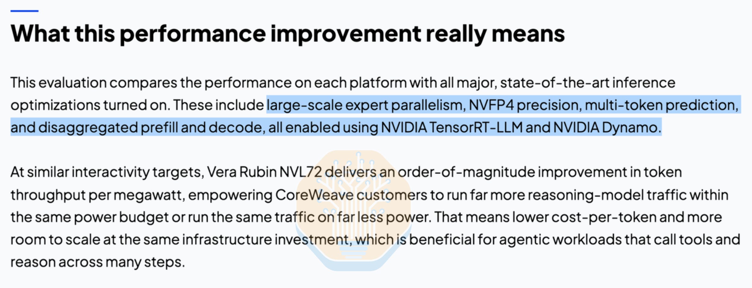
It is important to point out that CoreWeave claims to have enabled all of the following inference optimizations on both their baseline GB200 NVL72 and Rubin NVL72 performance results, including but not limited to:
NVFP4 Precision
Speculative Decoding (Using MTP)
Disaggregated Serving (Using Dynamo)
Wide Expert Parallelism
via TensorRT-LLM
The above results seem to suggest that Rubin comes to market with a strong performance gain vs Blackwell out of the gate. However, there are a few nuances that are worth unpacking.
First, attentive readers will note that CoreWeave is comparing Rubin against a GB200 NVL72 2025 baseline. In some ways, comparing performance at the early stages of GB200 NVL72’s lifecycle is fair, since Rubin performance is expected to massively improve from this early stage in its own lifecycle. Our analysis will also use the GB200 NVL72 early performance results from 2025, but we also compare how GB200 NVL72 did by 2026 as well as the most current GPU worth comparing to: GB300 NVL72. We will directly compare GB300 NVL72 performance from early in 2026 with Rubin’s comparable early lifecycle performance.

The second nuance in CoreWeave’s performance results is that they are using DeepSeek R1 671B, a model that is not widely used anymore. One would perhaps wish that CoreWeave used a more modern model like GLM5.2, Kimi K2.5, Qwen3.5, or DeepSeek V4. Even better would be Kimi K3 or Qwen3.8, both of which are coming soon to InferenceX! At least CoreWeave is not using GPTOSS 120B in Summer 2026 like AMD is for MI455X UALoE72 performance metrics. We expect that the fog of war created by benchmarking old models will be cleared up once Nvidia starts benchmarking Rubin on more modern model architectures with InferenceX in Q3 CY2026.
Oddly enough, CoreWeave’s choice of using DeepSeek R1 671B is theoretically more favourable towards the Blackwell baseline, and not Rubin. Rubin’s main advantages lie in a higher HBM capacity, higher CPU DRAM capacity, and greater HBM bandwidth, meaning that Rubin is more optimized for multi-trillion parameter models like Fable 5, Gemini Pro, Kimi K3, and Qwen3.8 2.4T.
The third noteworthy item is that CoreWeave uses only single turn 8k/1k input/output tokens. Theoretically, multi-turn long context workloads like Agentic Coding should do better on Rubin, due to Rubin’s higher HBM capacity and bandwidth, but this would not be captured on a simple single-turn benchmark. Our upcoming AgentX benchmark scenario created in collaboration with Weka, LMCache, the vLLM/SGLang community, Nvidia, AMD, and many others in the community will provide a realistic agentic workload to benchmark inference performance. We encourage everyone to adopt this inference benchmark!
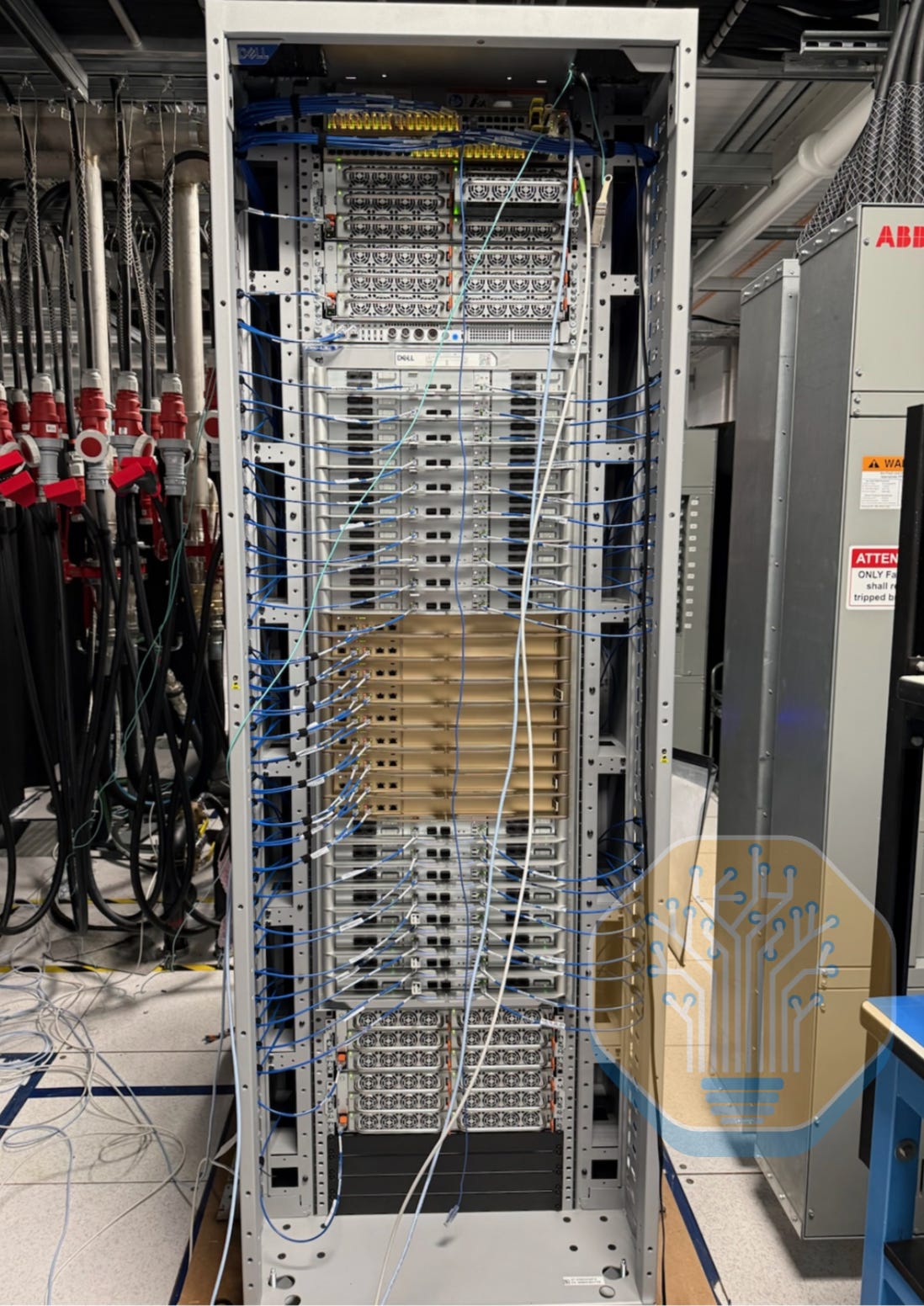
Finally, we note that CoreWeave’s testing was done on a pre-production rack without a scale-out fabric. Specifically, CoreWeave used a Dell Engineering Sample (ES) rack. We do believe these results are valuable as they use wide EP and PD disagg, which uses the NVL72 scale-up backplane and proves that it is working well. This backplane faced many reliability challenges during the ramp of GB200 NVL72 Oberon, as we have noted in our Accelerator model.
Rubin Versus Blackwell Performance per MegaWatt
The metric Nvidia chose to lead with was “output tokens per second per all-in utility megawatt”, counting every GPU in the system. To compare apples-to-apples, we renormalize our own InferenceX benchmark data onto the same total-GPU basis. Below, we put VR NVL72 up against our official GB200 and GB300 July 2026 benchmarks, as well as CoreWeave’s 2025 GB200 baseline.
The eye-catching multiples in Nvidia’s charts all come from the 2025 baseline. When comparing benchmark data, we believe we should use figures from the same time period, so the July 2026 GB200 and GB300 benchmarks are the more useful comparison.
In theory, datacenter PUE can be lower for Vera Rubin since Vera Rubin can operate with 45 degrees Celsius coolant temperatures in custom datacenters without chillers. However, for our comparisons, since most datacenters are designed to accommodate a wide variety of systems, we use the same PUE across the DLC cooled chips.
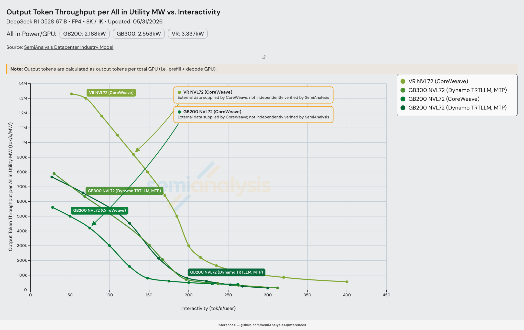
The following pareto curves plot output throughput per total-GPU megawatt against interactivity. Each line stops where its recipe’s frontier ends.
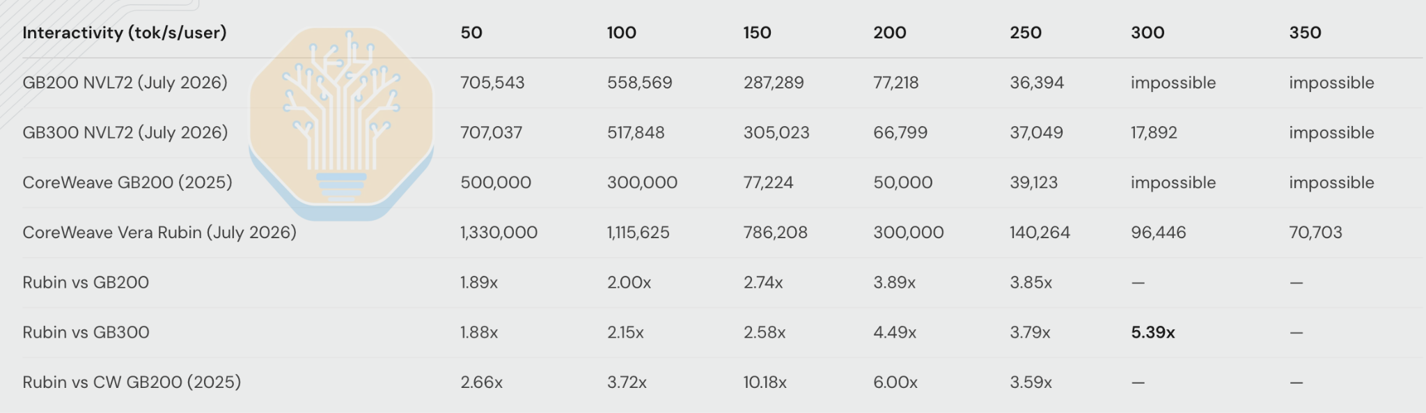
Next, we provide the same data in table form. When a cell says "impossible," we mean that the interactivity is past that recipe's frontier, simply not allowing the configuration to serve that workload at that speed.
Here is the same frontier as bars, across the 100 to 300 tok/s/user band. All four recipes have data through 250 tok/s/user, and only Rubin and GB300 make it to 300 tok/s/user.
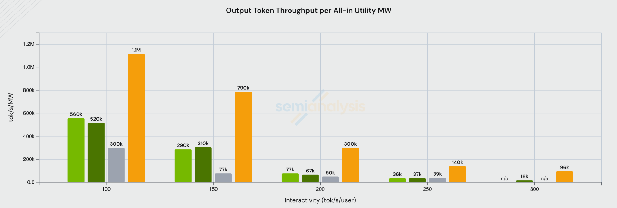

Let’s first compare Rubin against the July 2026 GB300 NVL72 baseline. Rubin’s lead is smallest at low interactivity and continues growing through the middle of the interactivity curve. Rubin sits at near 2x the throughput as Blackwell up through 100 tok/s/user, then widens to roughly 4x around 200 tok/s/user, where the gap peaks. Then, the gap begins to narrow again. The headline 5.4x performance gain over GB300 at 300 tok/s/user isn’t Rubin pulling further ahead. Rather, it is GB300 running the last, barely viable point on its frontier, which causes the ratio to balloon. GB200 can’t reach 300 tok/s/user at all. Blackwell’s per-GPU throughput drops off fast as the batch shrinks at high interactivity, while Rubin is still on a flatter part of its frontier.
Comparing Rubin against the 2025 GB200 NVL72 baseline is different, showing the biggest lead in the middle of the curve. The gap starts at under 3x at low speeds, but increasings to about 10x at 150 tok/s/user (the point Nvidia highlights in their chart), before falling back to 6x at around 200 tok/s/user. The data from that line is accurate, but as we have mentioned it use a software stack that is a year-old, not the GB200 you would run today.
At the very top of the interactivity range, the Blackwell curves drop off. By 350 tok/s/user, neither GB200 nor GB300 can serve the workloads at all, leaving only Rubin with an actual curve, delivering 96,446 tok/s/MW at 300 tok/s/user and 70,703 at 350 tok/s/user.
Clearly, Rubin is going to give us a lot more “fast mode” than Blackwell.
Rubin Versus Blackwell Performance per TCO
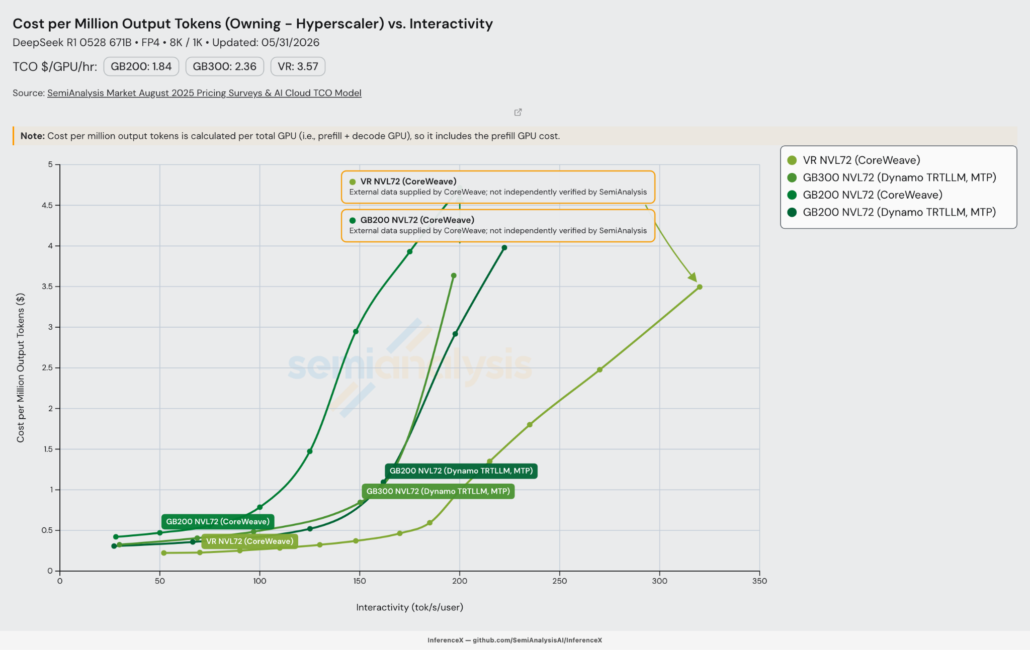
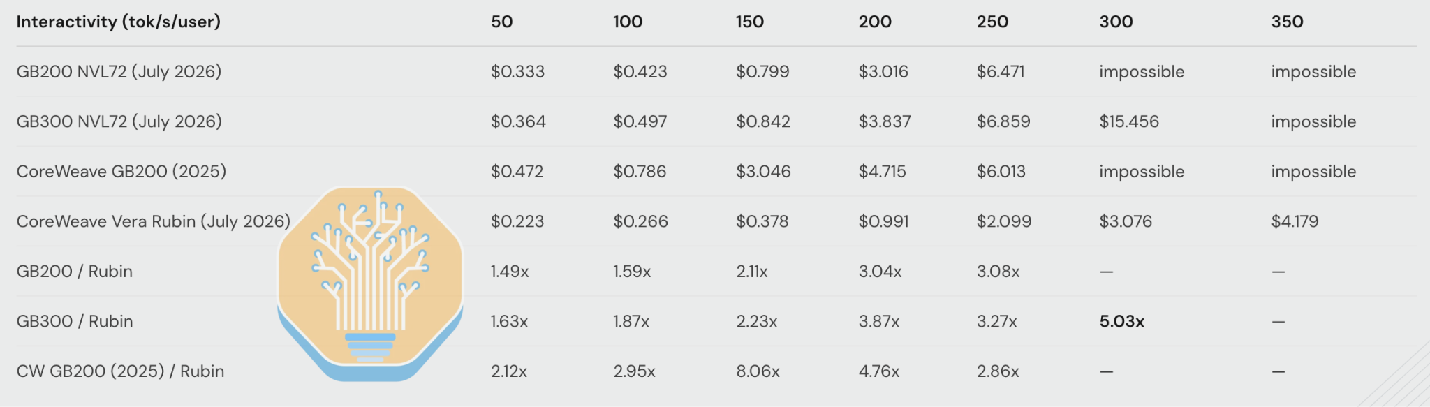
Per-megawatt performance only counts performance against power. Cost per million output tokens folds in the hardware’s total cost of ownership (TCO) including IT capital costs as well as electricity and datacenter costs. Our TCO model breaks this down comprehensively, providing capital costs and operating costs across server generations. Here, we divide each SKU's all-in TCO by that same renormalized output throughput, so lower is better. Rubin carries a higher TCO per GPU than Blackwell, $3.57 per GPU-hour against $1.84 for GB200 and $2.36 for GB300 in the operator ownership scenario (not rental prices). The charts and tables below will show how Rubin’s $ per token lead comes out a little smaller than its per-megawatt lead.

As with the per-MW analysis, the 2025 GB200 baseline produces the largest gains in performance for Rubin, but the July 2026 GB200 and GB300 numbers are the more relevant baseline for comparison for anyone buying capacity today.
The following pareto curves plot cost per million output tokens against interactivity. Each line stops where its recipe’s frontier ends.
Next, we provide the same data in table form, with the ratio showing how many times cheaper Rubin is at each interactivity. Again, a cell marked "impossible" is a speed that the recipe's frontier can't reach.
The chart below plots the frontier as bars across the 100 to 300 tok/s/user band. All four recipes have data through 250 tok/s/user, and only Rubin and GB300 reach 300 tok/s/user.
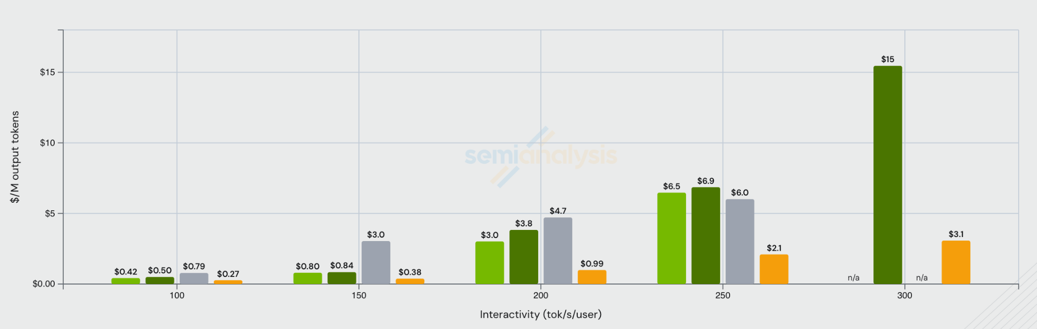

Against July 2026 GB200 & GB300, Rubin is cheaper at every interactivity, and the gap widens as you climb. The gap starts at about 1.5x cheaper than GB200 through 100 tok/s/user, and improves to 3x by 200 tok/s/user through to 250 tok/s/user. The 5x edge over GB300 at 300 tok/s/user is the same as the per-MW view, where GB300 can barely serve tokens and GB200 can’t serve at this interactivity level at all.
The 2025 GB200 NVL72 baseline is once again the more dramatic one, cresting in the middle of the curve. Rubin is a little over 2x cheaper at low speeds, peaks near 8x at 150 tok/s/user, and then moves back to 5x by 200 tok/s/user. Same comment as on the per-MW version: the 2025 GB200 baseline measures a year-old software stack, not the GB200 you would run today.
At the very top of the range, things are the same. GB200 has no operating point past 250 tok/s/user and GB300 has none past 300 tok/s/user, so by 350 tok/s/user only Rubin can serve at all, delivering a cost of $4.18 per million output tokens.
Below the paywall, we will continue breaking down Rubin’s performance as compared to the best-known publicly available MI355X distributed inferencing performance. We also briefly analyze how the Triton Compiler, PyTorch, vLLM, and Dynamo software will function on Rubin.